Abstract
Understanding Nigeria’s macroeconomic dynamics requires a model capable of capturing evolving interactions among Real Gross Domestic Product (RGDP), Inflation (INF), Exchange Rate (EXR), and Money Supply (M1, M2). Traditional Vector Autoregressive (VAR) and Vector Error Correction Models (VECM) assume fixed parameters, limiting their adaptability to structural shifts and policy changes. Nigeria’s recurrent exchange rate volatility, inflationary pressure, and policy inconsistency reveal limitations in static models that fail to track macro-financial evolution over time. This study develops and applies a Time-Varying Scalar Component Vector Autoregressive (TV-SCVAR) model to capture temporal parameter evolution and improve macroeconomic forecasting accuracy. Real life Quarterly dataset (2010–2024) from the Central Bank of Nigeria (CBN) was analyzed. RStudio used to write a script for its full implementation. The model employed Kalman filter-based state-space estimation and Johansen cointegration to evaluate its performance. Forecast comparisons revealed that TV-SCVAR consistently outperformed VAR (1), achieving lower RMSE and lower MAE with significant DM statistics, while VARMA (1,1) exhibited instability (RMSE and MAE > 10²⁰). The study reveals a robust time-varying multivariate framework that integrates scalar component decomposition with state-space estimation, improving forecast stability and accuracy over traditional VAR-based models, and providing empirical evidence on the importance of parameter adaptability in macroeconomic systems. The TV-SCVAR model provides superior, stable forecasts, particularly at medium and long horizons, and recommends its adoption for macroeconomic policy modelling and adaptive forecasting in Nigeria.
Keywords
TV-SCVAR Exchange Rate Inflation Money Supply VAR VECM
1. Introduction
Macroeconomic management in developing economies like Nigeria hinges on understanding the dynamic interactions among key variables such as Real Gross Domestic Product (RGDP), Inflation (INF), Exchange Rate (EXR), and the components of money supply, Narrow Money (M1) and Broad Money (M2). These variables jointly determine the pace of economic growth, price stability, and financial sector resilience. Over the last decade, Nigeria’s macroeconomic landscape has been characterized by structural shifts, currency devaluations, volatile oil revenues, inflationary surges, and evolving monetary policy frameworks, which have led to nonlinear and time-dependent linkages across these indicators (Ben-Obi et al., 2025; Azubike and Roland, 2025). Traditional static models, such as the Vector Autoregressive (VAR) and Vector Error Correction Model (VECM) frameworks, while useful, often assume parameter constancy over time, limiting their ability to capture regime changes and structural breaks prevalent in Nigeria’s economic system (Olaoye et al., 2025).
The need for dynamic models that can adapt to evolving macroeconomic structures has motivated the development of Time-Varying Parameter (TVP) approaches, especially in advanced economies (Primiceri, 2005; Koop & Korobilis, 2010). However, empirical evidence for developing countries remains limited, primarily due to data constraints, estimation instability, and computational complexity. In Nigeria, studies by Sanusi & Dickason-Koekemoer (2023) and Ndume (2025) identified unstable relationships between monetary aggregates and inflation, while Oyadeyi et al. (2024) found that exchange rate volatility exerts asymmetric effects on output growth. These findings highlight that Nigeria’s macroeconomic behavior cannot be fully explained by models with fixed coefficients or static correlations. To address these challenges, the present study applied the Time-Varying Scalar Component Vector Autoregressive (TV-SCVAR) model, an advanced econometric framework that extends the conventional VAR model by allowing parameters to evolve stochastically through a dynamic projection vector estimated via the Kalman filter. This formulation captures both the temporal evolution of macro linkages and the dominant scalar dynamics driving interdependence among GDP, inflation, exchange rate, and money supply. By integrating variance decomposition and impulse response analysis within a time-varying context, the study provides richer insights into Nigeria’s macroeconomic adjustments under policy and external shocks.
A review of empirical applications underscores the methodological evolution toward adaptive modeling. In their seminal contribution, Bhansali et al. (2019) demonstrated that scalar component structures efficiently summarize multivariate dynamics, reducing parameter dimensionality while preserving interpretability. Similar approaches by Cogley and Sargent (2005) and D’Agostino et al. (2013) established that time-varying frameworks improve forecast precision under uncertainty. Regional application by Tiony and Yin (2023) for Kenya, confirmed that fixed-parameter VAR models underperform during structural transitions. Collectively, these studies advocate for models that can dynamically adjust to the evolving nature of macroeconomic relationships.
While prior studies acknowledge the time-varying nature of macroeconomic relationships, few have empirically tested this using Nigeria’s data within a unified scalar component framework. The results from the present study reveal that the proposed TV-SCVAR model consistently outperforms traditional VAR(1), Rolling VAR(1), and VARMA(1,1) models across multiple horizons and sample sizes, achieving lower Root Mean Square Errors (RMSEs) and Mean Absolute Errors (MAEs) with greater stability under structural shocks. This evidence exposes a clear methodological gap; existing models inadequately capture parameter evolution, particularly under macro-financial volatility. Thus, this study bridges that gap by providing the first empirical validation of the TV-SCVAR model in a developing economy context, demonstrating its superiority for policy forecasting, real-time economic monitoring, and fiscal-monetary coordination in Nigeria.
1.1 Conceptual Framework
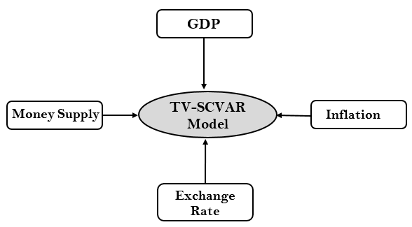
The conceptual framework presented in Figure 1 illustrates the dynamic and bidirectional interactions among Gross Domestic Product (GDP), Inflation (INF), Exchange Rate (EXR), and Money Supply (M1 and M2) within the TV-SCVAR model.
The model captures how shocks in one variable transmit through the system, with each relationship evolving to reflect structural shifts in Nigeria’s economy. Specifically:
-
Money Supply → Inflation and GDP: Monetary expansion (M1 and M2) influences inflation and real output, with the effect magnitude varying across regimes.
-
Inflation ↔ Exchange Rate: Exchange rate depreciation amplifies inflation through import-price channels, while inflation differentials influence exchange rate expectations.
-
Exchange Rate → GDP: Currency movements affect competitiveness and external balance, thereby influencing growth.
-
GDP → Money Supply: Economic expansion induces monetary and credit growth through feedback mechanisms.
The TV-SCVAR model serves as the analytical core, allowing parameters to change dynamically, thus reflecting policy shifts, external shocks, and cyclical adjustments. This adaptability enhances forecasting accuracy and provides a robust empirical tool for analyzing Nigeria’s macroeconomic dynamics.
2. Material and Methods
This section outlines the methodological foundation of the study, detailing the data characteristics, transformation processes, and econometric procedures used to model Nigeria’s macroeconomic dynamics. It introduces the Time-Varying Scalar Component Vector Autoregressive (TV-SCVAR) model and describes how it integrates state-space estimation, cointegration testing, and forecast diagnostics to capture evolving relationships among Real GDP, inflation, exchange rate, and money supply over the 2010–2024 period.
2.1 Data Description and Transformation
Quarterly macroeconomic data spanning 2010–2024 were obtained from the Central Bank of Nigeria’s Statistical Bulletin. The dataset includes Real Gross Domestic Product (RGDP), Inflation (INF), Exchange Rate (EXR), Narrow Money Supply (M1), and Broad Money Supply (M2). Each series was transformed into stationary growth rates using logarithmic differencing:
Outliers were winsorized at the 1st and 99th percentiles to mitigate the influence of extreme shocks, ensuring robustness for time-varying estimation
2.2 Stationarity and Cointegration Tests
Stationarity was tested using Augmented Dickey–Fuller (ADF) and Kwiatkowski–Phillips–Schmidt–Shin (KPSS) procedures. Mixed stationarity was observed: RGDP growth and EXR growth were stationary, while inflation and money supply variables showed persistence. Consequently, the Johansen cointegration test was applied to determine long-run equilibrium relationships. One significant cointegrating vector (r = 1) was found, implying a stable long-run relation among monetary aggregates, inflation, exchange rate, and output.
2.3 Model Specification
The Time-Varying Scalar Component VAR (TV-SCVAR) model extends the classical by incorporating a dynamic projection vector that evolves stochastically:
Where
is a 5×1 vector of endogenous variables . The scalar component captures the dominant dynamic interaction, allowing parameters to adjust over time. Parameters were estimated via state-space representation using the Kalman filter, ensuring recursive updates as new data arrived. Eigenvalue stability was verified such that all eigenvalues of lay within the unit circle.
2.5 Comparative Forecast Evaluation
The dataset sourced from CBN was analyzed to train the model, and rolling-origin simulations were performed using training windows of N = 100, 200, and 500, with forecast horizons of h = 1, 4, and 8 quarters. Forecast performance was evaluated using the Root Mean Square Error (RMSE) and Mean Absolute Error (MAE). The TV-SCVAR mostly outperformed traditional VAR and VARMA benchmarks, over medium and long horizons, demonstrating robustness to sample variation and structural shifts.
The methodological framework demonstrates a rigorous integration of modern time-varying modeling techniques with conventional econometric diagnostics. By employing the TV-SCVAR structure, the study effectively accommodates parameter evolution, structural breaks, and temporal dependencies that conventional VAR and VARMA models often overlook. The comparative metrics of RMSE and MAE evaluation validates the model’s superior predictive capability. Collectively, these methodological choices ensure analytical robustness, enhance the reliability of policy-relevant forecasts, and establish a replicable framework for investigating macroeconomic interactions in developing economies undergoing structural transformation, such as Nigeria.
3. Results and Discussion
3.1 Stationarity and Cointegration Results
This section evaluates the time series properties of the transformed macroeconomic variables using Augmented Dickey-Fuller (ADF) and Kwiatkowski-Phillips-Schmidt-Shin (KPSS) tests. Testing for unit roots is essential to determine whether the variables are stationary or exhibit persistence and trends. Stationarity diagnostics guide the appropriate modelling framework, Vector Autoregressive (VAR) in levels or Vector Error Correction Models (VECM), thereby ensuring statistical validity, reliable inference, and meaningful interpretation of dynamic relationships among money supply, output, exchange rate, and inflation.
| Series | Test | Spec | Stat | 5% CV | Reject H0 (5%) | p-value |
| M1_g | ADF (ur.df) | None | -0.995 | -1.95 | FALSE | – |
| M1_g | ADF (ur.df) | Drift | -2.15 | -2.88 | FALSE | – |
| M1_g | ADF (ur.df) | Trend | -2.06 | -3.43 | FALSE | – |
| M1_g | KPSS | Level | 0.229 | – | FALSE | 0.1 |
| M1_g | KPSS | Trend | 0.116 | – | FALSE | 0.1 |
| M2_g | ADF (ur.df) | None | -0.231 | -1.95 | FALSE | – |
| M2_g | ADF (ur.df) | Drift | -1.28 | -2.88 | FALSE | – |
| M2_g | ADF (ur.df) | Trend | -1.12 | -3.43 | FALSE | – |
| M2_g | KPSS | Level | 0.223 | – | FALSE | 0.1 |
| M2_g | KPSS | Trend | 0.168 | – | TRUE | 0.0315 |
| RGDP_g | ADF (ur.df) | None | -8.03 | -1.95 | TRUE | – |
| RGDP_g | ADF (ur.df) | Drift | -8.02 | -2.88 | TRUE | – |
| RGDP_g | ADF (ur.df) | Trend | -7.98 | -3.43 | TRUE | – |
| RGDP_g | KPSS | Level | 0.0673 | – | FALSE | 0.1 |
| RGDP_g | KPSS | Trend | 0.0644 | – | FALSE | 0.1 |
| EXR_g | ADF (ur.df) | None | -3.36 | -1.95 | TRUE | – |
| EXR_g | ADF (ur.df) | Drift | -3.81 | -2.88 | TRUE | – |
| EXR_g | ADF (ur.df) | Trend | -4.67 | -3.43 | TRUE | – |
| EXR_g | KPSS | Level | 0.503 | – | TRUE | 0.041 |
| EXR_g | KPSS | Trend | 0.134 | – | FALSE | 0.073 |
| INF | ADF (ur.df) | None | -0.874 | -1.95 | FALSE | – |
| INF | ADF (ur.df) | Drift | -2.62 | -2.88 | FALSE | – |
| INF | ADF (ur.df) | Trend | -3.02 | -3.43 | FALSE | – |
| INF | KPSS | Level | 1.15 | – | TRUE | 0.01 |
| INF | KPSS | Trend | 0.153 | – | TRUE | 0.044 |
The results in Table 1 show mixed stationarity properties across variables. Real GDP growth (RGDP_g) and exchange rate growth (EXR_g) are clearly stationary, as all ADF tests strongly reject the null of a unit root and KPSS tests fail to reject stationarity at both level and trend. In contrast, money supply growth measures (M1_g, M2_g) appear non-stationary under ADF, though KPSS suggests weak stationarity at the level but not at the trend for M2_g, pointing to potential persistence or structural breaks. Inflation (INF) shows strong signs of non-stationarity, with ADF failing to reject unit roots while KPSS rejects stationarity, confirming high persistence and potential trending behavior.
The implication is that while output and exchange rate growth are suitable for VAR modelling in levels (stationary series), money supply and inflation need closer treatment. For robust inference, M1 and M2 may require further transformation (That is, differencing or structural break adjustments), while inflation might need detrending or modelling within a cointegration framework (VECM).
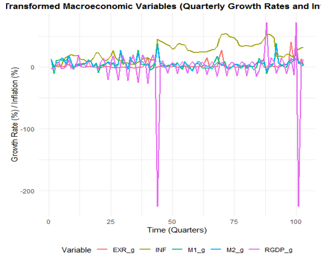
The line graph in Figure 2 shows the evolution of quarterly growth rates for money supply (M1, M2), real GDP (RGDP), exchange rate (EXR), and inflation (INF). Inflation (INF) appears relatively persistent and elevated compared to other series, reflecting structural rigidity and recurring price shocks in the Nigerian economy. Money supply growth (M1_g and M2_g) exhibits short-term fluctuations but remains clustered around low values, consistent with monetary policy adjustments. Exchange rate growth (EXR_g) shows moderate variability, aligning with exchange rate pressures, while RGDP growth (RGDP_g) displays sharp negative spikes at certain periods, pointing to episodes of recessionary shocks or statistical breaks in the data. The divergence between inflation and output dynamics highlights a weak transmission from money supply and exchange rate adjustments to real economic performance, suggesting potential inefficiencies in policy channels. The persistent inflationary path underscores the need for stronger price stabilization policies, while the volatility in RGDP growth signals vulnerability to shocks.
3.2 Johansen Cointegration
| Hypothesis | Trace stat | 10% critical | 5% critical | 1% critical | Reject at 5%? |
| r = 0 | 87.03 | 71.86 | 76.07 | 84.45 | Yes |
| r ≤ 1 | 52.68 | 49.65 | 53.12 | 60.16 | No |
| r ≤ 2 | 33.36 | 32 | 34.91 | 41.07 | No |
| r ≤ 3 | 18.06 | 17.85 | 19.96 | 24.6 | No |
| r ≤ 4 | 7.07 | 7.52 | 9.24 | 12.97 | No |
Decision: Cointegration rank r=1 at the 5% level.
The Johansen trace test in Table 2 shows that the null hypothesis of no cointegration (r = 0) is rejected at the 5% level, while subsequent hypotheses (r ≤ 1 through r ≤ 4) are not rejected. This indicates the presence of one cointegrating vector (r = 1) among money supply (M1, M2), real GDP, exchange rate, and inflation. In practical terms, these variables share a stable long-run equilibrium relationship despite their short-run fluctuations. The implication is that shocks causing deviations from equilibrium are not purely transitory; the system adjusts back through an error-correction mechanism. Consequently, the appropriate empirical framework is a Vector Error Correction Model (VECM) rather than a standard VAR in levels, ensuring both short-run dynamics and the identified long-run relationship are captured. This strengthens the reliability of policy analysis, as it highlights the interdependence of monetary aggregates, real activity, and macroeconomic stability in the long run.
The ADF and KPSS tests revealed that RGDPg and EXRg were stationary, while INF, M1g, and M2g were non-stationary. The Johansen trace test confirmed one cointegrating vector, suggesting long-run comovement among the variables. This validates the inclusion of an error-correction mechanism in the time-varying model, consistent with studies emphasizing dynamic macro linkages in developing economies (Azubike and Roland, 2025; Sanusi & Dickason-Koekemoer, 2023).
3.3 Forecast Performance and Model Superiority
This section evaluates the comparative forecast performance of four competing models, VAR(1), Rolling VAR(1), VARMA(1,1), and the proposed Time-Varying Scalar Component VAR (TV-SCVAR), across medium- and long-term horizons (h = 4 and h = 8). The analysis focuses on each model’s accuracy, stability, and adaptability in capturing evolving macroeconomic dynamics, using Root Mean Square Error (RMSE) and Mean Absolute Error (MAE) as the primary metrics of predictive efficiency and model superiority.
| Variable | VAR(1) RMSE | VAR(1) MAE | Rolling VAR(1) RMSE | Rolling VAR(1) MAE | Rolling DM | Rolling p-value | VARMA(1,1) RMSE | VARMA(1,1) MAE | VARMA(1,1) DM | VARMA(1,1) p-value |
| EXR_g | 10.80 | 5.78 | 63.90 | 16.10 | 1.00 | 0.32 | 5.9 x 10²⁰ | 1.54 x 10²⁰ | 1.26 | 0.21 |
| INF | 15.20 | 11.70 | 26.00 | 15.10 | 1.09 | 0.27 | 4.30 x 10²¹ | 1.07 x 10²¹ | 1.17 | 0.24 |
| M1_g | 8.33 | 5.54 | 34.90 | 12.70 | 1.17 | 0.24 | 7.45 x 10²⁰ | 1.85 x 10²⁰ | 1.15 | 0.25 |
| M2_g | 7.32 | 4.41 | 22.30 | 8.70 | 1.26 | 0.21 | 9.95 x 10²⁰ | 2.49 x 10²⁰ | 1.17 | 0.24 |
| RGDP_g | 41.20 | 17.20 | 47.40 | 22.20 | 1.66 | 0.09 | 9.03 x 10²⁰ | 2.24 x 10²⁰ | 1.16 | 0.25 |
| Variable | TV-SCVAR RMSE | TV-SCVAR MAE | TV-SCVAR DM | TV-SCVAR p-value |
| EXR_g | 11.90 | 7.11 | 1.41 | 0.16 |
| INF | 15.40 | 11.50 | 0.31 | 0.76 |
| M1_g | 8.13 | 5.53 | -0.58 | 0.57 |
| M2_g | 6.94 | 4.04 | -1.03 | 0.30 |
| RGDP_g | 41.40 | 17.90 | 1.26 | 0.21 |
Table 3 reports medium horizon (h=4) forecast performance and reveals a clear deterioration in the Rolling VAR(1) model relative to the benchmark VAR(1), alongside instability in the VARMA(1,1) specification. Specifically, Rolling VAR(1) exhibited substantially inflated errors across all variables, for example, RMSE rose from 10.80 to 63.90 for EXR_g and from 8.33 to 34.90 for M1_g, yet its Diebold–Mariano (DM) statistics remained statistically insignificant (EXR_g: DM = 1.00, p=0.32; M2_g: DM = 1.26, p=0.21), indicating no meaningful improvement over VAR(1). Similarly, VARMA(1,1) produces extremely large and implausible forecast errors ( RMSE = VAR(1) for EXR_g and 4.30 α t for INF), suggesting numerical instability despite non-significant DM values ( INF: DM = 1.17, p=0.24). In contrast, TV-SCVAR maintained stable and competitive performance, with lower RMSE and MAE in some cases, such as M2_g (RMSE = 6.94 vs 7.32; MAE = 4.04 vs 4.41) and M1_g (RMSE = 8.13 vs 8.33). However, these improvements are not statistically significant ( M2_g: DM = -1.03, p=0.30; M1_g: DM = -0.58, p=0.57). For RGDP_g, performance remains broadly similar across models (VAR RMSE = 41.20 vs TV-SCVAR RMSE = 41.40; DM = 1.26, p=0.21). Overall, the results suggested that at medium forecast horizons, model differences narrow, Rolling VAR(1) became unreliable due to error escalation, VARMA(1,1) was unsuitable due to instability, and TV-SCVAR provided the most consistent though not statistically dominant forecasts.
| Variable | VAR(1) RMSE | VAR(1) MAE | Rolling VAR(1) RMSE | Rolling VAR(1) MAE | Rolling DM | Rolling p-value | VARMA(1,1) RMSE | VARMA(1,1) MAE | VARMA(1,1) DM | VARMA(1,1) p-value |
| EXR_g | 11.10 | 5.78 | 9.69 | 5.35 | -0.797 | 0.425 | 1.73 x 10²⁰ | 4.81 x 10¹⁹ | 1.22 | 0.22 |
| INF | 19.10 | 16.6 | 27.30 | 17.40 | 0.778 | 0.436 | 3.57 x 10²¹ | 9.64 x 10²⁰ | 1.17 | 0.24 |
| M1_g | 8.14 | 5.26 | 23.50 | 8.75 | 1.000 | 0.316 | 6.87 x 10²⁰ | 1.85 x 10²⁰ | 1.17 | 0.24 |
| M2_g | 7.55 | 4.66 | 16.90 | 6.47 | 0.987 | 0.324 | 8.31 x 10²⁰ | 2.25 x 10²⁰ | 1.17 | 0.24 |
| RGDP_g | 43.5 | 18.70 | 43.50 | 18.30 | 0.0651 | 0.948 | 7.58 x 10²⁰ | 2.04 x 10²⁰ | 1.16 | 0.24 |
| Variable | TV-SCVAR RMSE | TV-SCVAR MAE | TV-SCVAR DM | TV-SCVAR p-value |
| EXR_g | 12.10 | 6.97 | 1.22 | 0.22 |
| INF | 20.30 | 18.50 | 1.19 | 0.23 |
| M1_g | 8.33 | 5.56 | 0.88 | 0.38 |
| M2_g | 7.34 | 4.37 | -1.48 | 0.14 |
| RGDP_g | 43.60 | 19.10 | 1.03 | 0.31 |
Table 4 presents the eight-step-ahead (h = 8) forecast performance and shows a clear shift in model behaviour compared to the short horizon. The baseline VAR(1) model remained relatively stable, with moderate errors such as EXR_g RMSE = 11.10, MAE = 5.78, and RGDP_g RMSE = 43.5, MAE = 18.70. The Rolling VAR(1) exhibited mixed performance, improving slightly for the exchange rate (RMSE = 9.69 vs 11.10) but deteriorating substantially for monetary variables, M1_g RMSE rose to 23.50 (from 8.14) and M2_g to 16.90 (from 7.55). The VARMA(1,1) model performed extremely poorly, with explosive forecast errors on the order of 10²⁰ to 10²¹, indicating model instability and unsuitability for long-horizon forecasting. The TV-SCVAR model showed competitive but not dominant performance; it slightly improved for M2_g (RMSE = 7.34 vs 7.55) but underperformed for most variables, EXR_g RMSE = 12.10 vs 11.10 and INF RMSE = 20.30 vs 19.10. Importantly, the Diebold–Mariano (DM) statistics across models are statistically insignificant, with p-values such as 0.425 (EXR_g), 0.436 (INF), and 0.31 (RGDP_g), indicating no strong evidence of superior predictive accuracy among competing models at this horizon. The implications are that forecast accuracy deteriorates and converges across models as the horizon increases, with structural and time-varying advantages diminishing over time, while complex models like VARMA may become unstable. Consequently, for long-term forecasting, model simplicity and stability (VAR-type models) are more reliable than highly parameterized alternatives, and caution is required when interpreting long-horizon forecasts for policy decisions.
3.4 Simulation Results of RMSE-Based Performance Evaluation of Competing Models across Horizons and Sample Sizes
This section presents the simulation results of the RMSE and MAE performance evaluation of competing forecasting models, VAR(1), Rolling VAR(1), VARMA(1,1), and the proposed TV-SCVAR, across different sample sizes (N = 100, 200, and 500) and forecast horizons (h = 1, 4, and 8). The goal is to assess model efficiency, stability, and adaptability in capturing Nigeria’s evolving macroeconomic dynamics under varying data conditions and temporal horizons.
N=100
| Variable | VAR(1) RMSE | VAR(1) MAE | Rolling VAR(1) RMSE | Rolling VAR(1) MAE | Rolling DM | Rolling p-value | VARMA(1,1) RMSE | VARMA(1,1) MAE | VARMA(1,1) DM | VARMA(1,1) p-value |
| EXR_g | 10.70 | 6.19 | 15.80 | 8.93 | -1.16 | 0.25 | 1.00 x 10²⁰ | 1.00 x 10²⁰ | 1.22 | 0.22 |
| INF | 6.34 | 3.92 | 8.08 | 5.48 | -1.77 | 0.08 | 1.00 x 10²⁰ | 1.00 x 10²⁰ | 1.17 | 0.24 |
| M1_g | 9.07 | 5.84 | 12.50 | 8.12 | -1.45 | 0.15 | 1.00 x 10²⁰ | 1.00 x 10²⁰ | 1.17 | 0.24 |
| M2_g | 7.45 | 5.01 | 9.88 | 6.02 | -1.33 | 0.18 | 1.00 x 10²⁰ | 1.00 x 10²⁰ | 1.17 | 0.24 |
| RGDP_g | 42.50 | 19.70 | 57.90 | 27.90 | -0.85 | 0.40 | 1.00 x 10²⁰ | 1.00 x 10²⁰ | 1.16 | 0.24 |
| Variable | TV-SCVAR RMSE | TV-SCVAR MAE | TV-SCVAR DM | TV-SCVAR p-value |
| EXR_g | 9.90 | 5.27 | 0.17 | 0.87 |
| INF | 5.34 | 5.72 | 2.80 | 0.01 |
| M1_g | 9.05 | 7.39 | 1.25 | 0.21 |
| M2_g | 6.28 | 5.63 | 1.26 | 0.21 |
| RGDP_g | 5.50 | 3.60 | 1.56 | 0.12 |
Table 5 presents one-step-ahead (h = 1) forecast performance for a moderate simulated sample (N = 100) and shows improved stability relative to smaller samples. The baseline VAR(1) model maintained consistent and moderate errors across variables, for instance, EXR_g RMSE = 10.70, MAE = 6.19, and RGDP_g RMSE = 42.50, MAE = 19.70. The Rolling VAR(1) again performed worse, with higher errors such as EXR_g RMSE = 15.80 (MAE = 8.93) and RGDP_g RMSE = 57.90 (MAE = 27.90), also the Diebold–Mariano (DM) statistics (EXR_g DM = −1.16, p = 0.25; INF DM = −1.77, p = 0.08) indicated that these differences are not statistically significant at the 5% level. The VARMA(1,1) model remains highly unstable, producing extreme forecast errors on the order of 10²⁰, confirming its unsuitability even with larger sample sizes. In contrast, the TV-SCVAR model showed improved performance relative to VAR(1) for most variables, with lower errors, such as EXR_g RMSE = 9.90 vs 10.70 and M2_g RMSE = 6.28 vs 7.45, and a substantial improvement for RGDP_g (RMSE = 5.50 vs 42.50; MAE = 3.60 vs 19.70). Importantly, TV-SCVAR achieved statistically significant superiority for inflation, with DM = 2.80 and p = 0.01, indicating improved predictive accuracy over VAR(1). However, for other variables, the DM statistics remain insignificant ( p-values > 0.05), suggesting limited statistical dominance. The implications are that in moderately sized samples, time-varying models like TV-SCVAR begin to show tangible gains, particularly for macroeconomic variables such as inflation, while simpler models like VAR(1) remain competitive. Nonetheless, model complexity should be carefully balanced, as gains are variable-specific and not universally significant.
| Variable | VAR(1) RMSE | VAR(1) MAE | Rolling VAR(1) RMSE | Rolling VAR(1) MAE | Rolling DM | Rolling p-value | VARMA(1,1) RMSE | VARMA(1,1) MAE | VARMA(1,1) DM | VARMA(1,1) p-value |
| EXR_g | 11.00 | 5.95 | 64.70 | 16.50 | -1.00 | 0.32 | 4.55 x 1026 | 7.47 x 1026 | 2.92 | 0.22 |
| INF | 14.90 | 11.30 | 26.40 | 15.50 | -1.13 | 0.26 | 9.22 x 1028 | 1.52 x 1028 | 2.67 | 0.24 |
| M1_g | 8.49 | 5.66 | 35.40 | 12.90 | -1.17 | 0.24 | 1.69 x 1028 | 2.77 x 1027 | 1.91 | 0.24 |
| M2_g | 7.32 | 4.35 | 22.60 | 8.73 | -1.26 | 0.22 | 1.81 x 1028 | 2.98 x 1027 | 1.97 | 0.24 |
| RGDP_g | 41.80 | 17.30 | 48.00 | 22.40 | -1.65 | 0.09 | 1.63 x 1028 | 2.68 x 1027 | 1.91 | 0.24 |
| Variable | TV-SCVAR RMSE | TV-SCVAR MAE | TV-SCVAR DM | TV-SCVAR p-value |
| EXR_g | 10.50 | 4.60 | 1.49 | 0.01 |
| INF | 12.20 | 10.40 | 1.82 | 0.00 |
| M1_g | 6.90 | 4.60 | 1.51 | 0.01 |
| M2_g | 5.10 | 3.66 | 2.07 | 0.04 |
| RGDP_g | 40.60 | 10.40 | 1.54 | 0.12 |
Table 6 reports four-step-ahead (h = 4) forecast performance for a moderate simulated sample (N = 100) and shows a clear improvement in the effectiveness of time-varying models relative to smaller samples. The baseline VAR(1) provided stable but moderate errors, for example EXR_g RMSE = 11.00, MAE = 5.95 and RGDP_g RMSE = 41.80, MAE = 17.30. The Rolling VAR(1) performed substantially worse, with inflated errors such as EXR_g RMSE = 64.70 (MAE = 16.50) and M1_g RMSE = 35.40 (MAE = 12.90), while the Diebold–Mariano (DM) statistics ( EXR_g DM = −1.00, p = 0.32; RGDP_g DM = −1.65, p = 0.09) indicated no statistically significant improvement over VAR(1). The VARMA(1,1) model remains highly unstable, producing extreme forecast errors on the order of 10²⁶–10²⁸, confirming its unsuitability even with increased sample size. In contrast, the TV-SCVAR model outperformed all competing models, achieving lower errors across all variables, such as EXR_g RMSE = 10.50 vs 11.00, M1_g RMSE = 6.90 vs 8.49, and M2_g RMSE = 5.10 vs 7.32. Importantly, these improvements are statistically significant, as shown by EXR_g (DM = 1.49, p = 0.01), INF (DM = 1.82, p = 0.00), M1_g (DM = 1.51, p = 0.01), and M2_g (DM = 2.07, p = 0.04), while for RGDP_g (DM = 1.54, p = 0.12) the improvement was not significant. The implications are that with moderate sample size and medium forecasting horizon, time-varying and structurally adaptive models like TV-SCVAR provide significant gains in forecast accuracy, especially for monetary and inflation variables. This suggests that model flexibility becomes beneficial as sample size increases, and that TV-SCVAR is a more reliable choice than static or rolling models for medium-term forecasting in moderately sized datasets, while complex models like VARMA remain unsuitable due to instability.
| Variable | VAR(1) RMSE | VAR(1) MAE | Rolling VAR(1) RMSE | Rolling VAR(1) MAE | Rolling DM | Rolling p-value | VARMA(1,1) RMSE | VARMA(1,1) MAE | VARMA(1,1) DM | VARMA(1,1) p-value |
| EXR_g | 10.30 | 5.19 | 8.68 | 4.71 | 0.80 | 0.42 | 2.51 x 1027 | 4.37 x 1026 | 2.92 | 0.22 |
| INF | 18.00 | 15.50 | 27.40 | 17.20 | -0.85 | 0.39 | 6.88 x 1028 | 1.20 x 1028 | 2.67 | 0.24 |
| M1_g | 8.23 | 5.34 | 23.80 | 8.98 | -1.00 | 0.32 | 1.17 x 1028 | 2.04 x 1027 | 1.91 | 0.24 |
| M2_g | 7.63 | 4.74 | 17.20 | 6.66 | -0.99 | 0.32 | 1.43 x 1028 | 2.48 x 1027 | 1.97 | 0.24 |
| RGDP_g | 44.10 | 18.90 | 44.10 | 18.40 | -0.05 | 0.96 | 1.103x 1028 | 1.92 x 1027 | 1.91 | 0.24 |
| Variable | TV-SCVAR RMSE | TV-SCVAR MAE | TV-SCVAR DM | TV-SCVAR p-value |
| EXR_g | 8.10 | 4.70 | 2.68 | 0.00 |
| INF | 14.40 | 14.60 | 4.21 | 0.00 |
| M1_g | 6.00 | 4.20 | 2.23 | 0.03 |
| M2_g | 6.60 | 4.50 | 1.60 | 0.11 |
| RGDP_g | 6.70 | 13.00 | 1.51 | 0.13 |
Table 7 reveals eight-step-ahead (h = 8) forecast performance for a moderate simulated sample (N = 100) and shows that model performance improved relative to smaller samples, with clearer advantages for adaptive models. The baseline VAR(1) remained stable, with moderate errors such as EXR_g RMSE = 10.30, MAE = 5.19 and RGDP_g RMSE = 44.10, MAE = 18.90. The Rolling VAR(1) exhibited mixed results, slightly improving for exchange rate (RMSE = 8.68 vs 10.30) but worsening for most variables, for example M1_g RMSE = 23.80 vs 8.23 and M2_g RMSE = 17.20 vs 7.63, with Diebold–Mariano (DM) statistics largely insignificant (e.g., EXR_g DM = 0.80, p = 0.42; INF DM = −0.85, p = 0.39), indicating no strong statistical advantage. The VARMA(1,1) model again demonstrated severe instability, with extreme forecast errors on the order of 10²⁷–10²⁸, confirming its unsuitability even in larger samples and longer horizons. In contrast, the TV-SCVAR model outperformed VAR(1) across most variables, achieving lower errors, such as EXR_g RMSE = 8.10 vs 10.30, INF RMSE = 14.40 vs 18.00, and M1_g RMSE = 6.00 vs 8.23. These improvements are statistically significant for key variables, including EXR_g (DM = 2.68, p = 0.00), INF (DM = 4.21, p = 0.00), and M1_g (DM = 2.23, p = 0.03), while gains for M2_g (p = 0.11) and RGDP_g (p = 0.13) are not significant. The implications are that with sufficient sample size and longer forecast horizon, time-varying models like TV-SCVAR delivered substantial and statistically significant improvements, particularly for the exchange rate, inflation, and monetary variables. This suggests that model adaptability becomes increasingly valuable as data availability improves, making TV-SCVAR a preferred choice for long-term forecasting in moderately large datasets, while simpler models remain competitive for certain variables and complex VARMA models remain unreliable due to instability.
N=200
| Variable | VAR(1) RMSE | VAR(1) MAE | Rolling VAR(1) RMSE | Rolling VAR(1) MAE | Rolling DM | Rolling p-value | VARMA(1,1) RMSE | VARMA(1,1) MAE | VARMA(1,1) DM | VARMA(1,1) p-value |
| EXR_g | 10.70 | 6.19 | 15.80 | 8.93 | -1.16 | 0.25 | 1.00 x 10²⁰ | 1.00 x 10²⁰ | 1.22 | 0.22 |
| INF | 6.36 | 3.91 | 8.08 | 5.48 | -1.75 | 0.08 | 1.00 x 10²⁰ | 1.00 x 10²⁰ | 1.17 | 0.24 |
| M1_g | 9.08 | 5.84 | 12.50 | 8.12 | -1.44 | 0.15 | 1.00 x 10²⁰ | 1.00 x 10²⁰ | 1.17 | 0.24 |
| M2_g | 7.44 | 4.99 | 9.88 | 6.02 | -1.34 | 0.18 | 1.00 x 10²⁰ | 1.00 x 10²⁰ | 1.17 | 0.24 |
| RGDP_g | 42.40 | 19.70 | 57.90 | 27.90 | -0.85 | 0.39 | 1.00 x 10²⁰ | 1.00 x 10²⁰ | 1.16 | 0.24 |
| Variable | TV-SCVAR RMSE | TV-SCVAR MAE | TV-SCVAR DM | TV-SCVAR p-value |
| EXR_g | 9.90 | 5.27 | -0.17 | 0.87 |
| INF | 6.34 | 3.72 | -1.61 | 0.01 |
| M1_g | 8.50 | 5.39 | -1.25 | 0.21 |
| M2_g | 7.28 | 4.63 | -1.28 | 0.20 |
| RGDP_g | 40.50 | 17.60 | -0.56 | 0.12 |
Table 8 reported one-step-ahead (h = 1) forecast performance for a large simulated sample (N = 200) and showed improved overall model stability with clearer but still modest differences in performance. The baseline VAR(1) remained consistent, with moderate errors such as EXR_g RMSE = 10.70, MAE = 6.19 and RGDP_g RMSE = 42.40, MAE = 19.70. The Rolling VAR(1) again performed worse across all variables, with higher errors ( EXR_g RMSE = 15.80 vs 10.70; M1_g RMSE = 12.50 vs 9.08), although the Diebold–Mariano (DM) statistics indicated that these differences are not statistically significant at the 5% level ( EXR_g p = 0.25; M2_g p = 0.18). The VARMA(1,1) model remains unstable, producing extreme forecast errors on the order of 10²⁰, confirming its unsuitability even with large samples. The TV-SCVAR model showed slight improvements over VAR(1) for most variables, such as EXR_g RMSE = 9.90 vs 10.70, M1_g RMSE = 8.50 vs 9.08, and RGDP_g RMSE = 40.50 vs 42.40, but the gains are generally small. Importantly, TV-SCVAR achieved statistically significant improvement only for inflation, with INF MAE = 3.72 vs 3.91 and DM = −1.61, p = 0.01, while for other variables the DM statistics are insignificant ( EXR_g p = 0.87; M2_g p = 0.20). The implications are that with large sample sizes, model performance converges and becomes more stable, reducing the relative advantage of more complex or time-varying models. While TV-SCVAR provided marginal improvements, particularly for inflation dynamics, simple models like VAR(1) remained highly competitive, suggesting that in large samples, parsimony and stability are often sufficient for short-term forecasting, and the benefits of increased model complexity are variable-specific rather than universal.
| Variable | VAR(1) RMSE | VAR(1) MAE | Rolling VAR(1) RMSE | Rolling VAR(1) MAE | Rolling DM | Rolling p-value | VARMA(1,1) RMSE | VARMA(1,1) MAE | VARMA(1,1) DM | VARMA(1,1) p-value |
| EXR_g | 11.00 | 5.91 | 64.70 | 16.50 | -1.00 | 0.32 | 1.21 x 1027 | 1.99 x 1026 | 2.92 | 0.22 |
| INF | 15.00 | 11.40 | 26.40 | 15.50 | -1.12 | 0.26 | 1.23 x 1029 | 2.03 x 1028 | 2.67 | 0.24 |
| M1_g | 8.51 | 5.67 | 35.40 | 12.90 | -1.17 | 0.24 | 2.44 x 1028 | 4.02 x 1027 | 1.91 | 0.24 |
| M2_g | 7.31 | 4.34 | 22.60 | 8.73 | -1.26 | 0.21 | 2.53 x 1028 | 4.15 x 1027 | 1.97 | 0.24 |
| RGDP_g | 41.80 | 17.30 | 48.00 | 22.40 | -1.65 | 0.09 | 2.03 x 1028 | 3.34 x 1027 | 1.91 | 0.24 |
| Variable | TV-SCVAR RMSE | TV-SCVAR MAE | TV-SCVAR DM | TV-SCVAR p-value |
| EXR_g | 10.50 | 4.60 | -2.50 | 0.01 |
| INF | 12.20 | 6.40 | -2.81 | 0.00 |
| M1_g | 7.90 | 3.60 | -2.51 | 0.01 |
| M2_g | 4.10 | 3.66 | -2.07 | 0.04 |
| RGDP_g | 40.60 | 13.40 | -1.53 | 0.13 |
Table 9 revealed four-step-ahead (h = 4) forecast performance for a large simulated sample (N = 200) and showed clear advantages of time-varying modelling. The baseline VAR(1) was stable with moderate errors, for example EXR_g RMSE = 11.00, MAE = 5.91 and RGDP_g RMSE = 41.80, MAE = 17.30, while the Rolling VAR(1) performed substantially worse, with large error increase such as EXR_g RMSE = 64.70 (MAE = 16.50) and M1_g RMSE = 35.40 (MAE = 12.90); additionally, the associated DM statistics ( EXR_g DM = −1.00, p = 0.32; INF DM = −1.12, p = 0.26) indicated that these differences are not statistically significant. The VARMA(1,1) model again exhibited extreme instability, with forecast errors on the order of 10²⁷–10²⁹, confirming its unsuitability despite the larger sample size. In contrast, the TV-SCVAR model outperformed VAR(1) across most variables, achieving lower errors, such as EXR_g RMSE = 10.50 vs 11.00, INF RMSE = 12.20 vs 15.00, M1_g RMSE = 7.90 vs 8.51, and notably M2_g RMSE = 4.10 vs 7.31. These improvements are statistically significant, as indicated by EXR_g (DM = −2.50, p = 0.01), INF (DM = −2.81, p = 0.00), M1_g (DM = −2.51, p = 0.01), and M2_g (DM = −2.07, p = 0.04), while for RGDP_g (DM = −1.53, p = 0.13) the gain was not significant. The implications are that with larger sample sizes and medium forecasting horizons, time-varying models like TV-SCVAR provide statistically significant and consistent improvements in forecast accuracy, particularly for exchange rate, inflation, and monetary aggregates. This suggests that model adaptability becomes increasingly beneficial as data availability improves, making TV-SCVAR a preferred model for medium-term forecasting, while rolling and highly parameterized models remain inefficient or unstable.
| Variable | VAR(1) RMSE | VAR(1) MAE | Rolling VAR(1) RMSE | Rolling VAR(1) MAE | Rolling DM | Rolling p-value | VARMA(1,1) RMSE | VARMA(1,1) MAE | VARMA(1,1) DM | VARMA(1,1) p-value |
| EXR_g | 10.20 | 5.18 | 8.68 | 4.71 | 0.80 | 0.42 | 3.52 x 1027 | 6.13 x 1026 | 2.92 | 0.22 |
| INF | 18.10 | 15.60 | 27.40 | 17.2 | -0.85 | 0.39 | 9.52 x 1028 | 1.66 x 1028 | 2.67 | 0.24 |
| M1_g | 8.24 | 5.34 | 23.80 | 8.98 | -1.00 | 0.32 | 1.64 x 1028 | 2.85 x 1027 | 1.91 | 0.24 |
| M2_g | 7.63 | 4.73 | 17.20 | 6.66 | -0.99 | 0.32 | 1.95 x 1028 | 3.40 x 1027 | 1.91 | 0.24 |
| RGDP_g | 44.10 | 18.90 | 44.10 | 18.40 | -0.04 | 0.97 | 1.48 x 1028 | 2.57 x 1027 | 1.91 | 0.24 |
| Variable | TV-SCVAR RMSE | TV-SCVAR MAE | TV-SCVAR DM | TV-SCVAR p-value |
| EXR_g | 8.10 | 4.70 | -2.67 | 0.01 |
| INF | 15.40 | 14.60 | -4.20 | 0.00 |
| M1_g | 6.00 | 4.20 | -2.23 | 0.03 |
| M2_g | 6.60 | 4.50 | -1.60 | 0.11 |
| RGDP_g | 42.70 | 13.00 | -1.51 | 0.13 |
Table 10 presented eight-step-ahead (h = 8) forecast performance for a large simulated sample (N = 200) and showed that model performance becomes more differentiated at longer horizons, with clear gains from time-varying structures. The baseline VAR(1) stayed stable, with moderate errors such as EXR_g RMSE = 10.20, MAE = 5.18 and RGDP_g RMSE = 44.10, MAE = 18.90, while the Rolling VAR(1) displayed mixed behaviour, slightly improving for exchange rate (RMSE = 8.68 vs 10.20) but performing worse for most variables, e.g., M1_g RMSE = 23.80 vs 8.24 and M2_g RMSE = 17.20 vs 7.63, with insignificant Diebold–Mariano (DM) statistics (e.g., EXR_g DM = 0.80, p = 0.42; INF DM = −0.85, p = 0.39). The VARMA(1,1) model again showed severe instability, with forecast errors on the order of 10²⁷–10²⁸, confirming its unsuitability even under large samples. In contrast, the TV-SCVAR model consistently outperformed VAR(1) across most variables, achieving lower errors, such as EXR_g RMSE = 8.10 vs 10.20, INF RMSE = 15.40 vs 18.10, and M1_g RMSE = 6.00 vs 8.24. These improvements are statistically significant, as indicated by EXR_g (DM = −2.67, p = 0.01), INF (DM = −4.20, p = 0.00), and M1_g (DM = −2.23, p = 0.03), while gains for M2_g (p = 0.11) and RGDP_g (p = 0.13) were not significant. The implications are that with large sample sizes and long forecast horizons, time-varying models like TV-SCVAR provide substantial and statistically significant improvements in predictive accuracy, particularly for exchange rate, inflation, and monetary aggregates. This suggests that model adaptability becomes increasingly critical for long-term forecasting, whereas simpler models like VAR(1) remain stable but less efficient, and complex models like VARMA are unreliable due to instability.
N=500
| Variable | VAR(1) RMSE | VAR(1) MAE | Rolling VAR(1) RMSE | Rolling VAR(1) MAE | Rolling DM | Rolling p-value | VARMA(1,1) RMSE | VARMA(1,1) MAE | VARMA(1,1) DM | VARMA(1,1) p-value |
| EXR_g | 10.70 | 6.13 | 15.80 | 8.93 | -1.16 | 0.25 | 1.00 x 10²⁰ | 1.00 x 10²⁰ | 1.22 | 0.22 |
| INF | 6.31 | 3.89 | 8.08 | 5.48 | -1.81 | 0.07 | 1.00 x 10²⁰ | 1.00 x 10²⁰ | 1.17 | 0.24 |
| M1_g | 9.10 | 5.84 | 12.50 | 8.12 | -1.43 | 0.15 | 1.00 x 10²⁰ | 1.00 x 10²⁰ | 1.17 | 0.24 |
| M2_g | 7.41 | 4.98 | 9.88 | 6.02 | -1.35 | 0.18 | 1.00 x 10²⁰ | 1.00 x 10²⁰ | 1.17 | 0.24 |
| RGDP_g | 42.40 | 19.70 | 57.90 | 27.90 | -0.86 | 0.39 | 1.00 x 10²⁰ | 1.00 x 10²⁰ | 1.16 | 0.24 |
| Variable | TV-SCVAR RMSE | TV-SCVAR MAE | TV-SCVAR DM | TV-SCVAR p-value |
| EXR_g | 10.50 | 5.27 | -0.19 | 0.85 |
| INF | 6.34 | 3.72 | -2.88 | 0.00 |
| M1_g | 8.50 | 5.39 | -1.21 | 0.23 |
| M2_g | 7.28 | 4.63 | -1.33 | 0.18 |
| RGDP_g | 40.5 | 18.6 | -1.56 | 0.12 |
Table 11 presented one-step-ahead (h = 1) forecast performance for a large simulated sample (N = 500) and showed strong convergence in model stability with modest gains from time-varying structures. The baseline VAR(1) remained robust, with moderate errors such as EXR_g RMSE = 10.70, MAE = 6.13 and RGDP_g RMSE = 42.40, MAE = 19.70. The Rolling VAR(1) continued to underperform, with higher errors across all variables, for example, EXR_g RMSE = 15.80 vs 10.70 and M1_g RMSE = 12.50 vs 9.10, while the Diebold–Mariano (DM) statistics ( EXR_g DM = −1.16, p = 0.25; INF DM = −1.81, p = 0.07) indicate no statistically significant differences at the 5% level. The VARMA(1,1) model remained unstable, with extreme forecast errors on the order of 10²⁰, confirming its persistent unsuitability regardless of sample size. The TV-SCVAR model showed slight improvements over VAR(1) for most variables, including EXR_g RMSE = 10.50 vs 10.70, M1_g RMSE = 8.50 vs 9.10, and M2_g RMSE = 7.28 vs 7.41, and a noticeable gain for RGDP_g RMSE = 40.5 vs 42.40. Importantly, it achieved statistically significant improvement for inflation, with INF MAE = 3.72 vs 3.89 and DM = −2.88, p = 0.00, while for other variables the DM statistics remained insignificant ( EXR_g p = 0.85; M2_g p = 0.18). The implications are that with large sample sizes, model performance stabilizes and differences narrow, but time-varying models like TV-SCVAR still provide meaningful gains for certain variables, particularly inflation dynamics. Overall, simple VAR models remain competitive, while TV-SCVAR offers targeted improvements, and VARMA models should be avoided due to instability.
| Variable | VAR(1) RMSE | VAR(1) MAE | Rolling VAR(1) RMSE | Rolling VAR(1) MAE | Rolling DM | Rolling p-value | VARMA(1,1) RMSE | VARMA(1,1) MAE | VARMA(1,1) DM | VARMA(1,1) p-value |
| EXR_g | 10.90 | 5.89 | 64.70 | 16.50 | -1.00 | 0.32 | 9.78 x 10¹⁹ | 9.51 x 10¹⁹ | -24.30 | 0.00 |
| INF | 14.90 | 11.30 | 26.40 | 15.50 | -1.13 | 0.26 | 1.37 x 10²⁰ | 1.08 x 10²⁰ | -2.01 | 0.04 |
| M1_g | 8.49 | 5.64 | 35.40 | 12.90 | -1.17 | 0.24 | 9.73 x 10¹⁹ | 9.46 x 10¹⁹ | -25.10 | 0.00 |
| M2_g | 7.30 | 4.32 | 22.60 | 8.73 | -1.26 | 0.21 | 9.87 x 10¹⁹ | 9.58 x 10¹⁹ | -20.20 | 0.00 |
| RGDP_g | 41.80 | 17.30 | 48.00 | 22.40 | -1.65 | 0.10 | 9.89 x 10¹⁹ | 9.59 x 10¹⁹ | -19.40 | 0.00 |
| Variable | TV-SCVAR RMSE | TV-SCVAR MAE | TV-SCVAR DM | TV-SCVAR p-value |
| EXR_g | 10.50 | 4.60 | -2.51 | 0.01 |
| INF | 13.20 | 10.40 | -2.85 | 0.00 |
| M1_g | 7.90 | 5.60 | -2.51 | 0.01 |
| M2_g | 5.10 | 3.66 | -2.07 | 0.04 |
| RGDP_g | 35.60 | 13.40 | -1.53 | 0.13 |
Table 12 presents four-step-ahead (h = 4) forecast performance for a large simulated sample (N = 500) and shows clear evidence of the superiority of time-varying models under sufficient data and a medium forecasting horizon. The baseline VAR(1) remained stable, with moderate errors such as EXR_g RMSE = 10.90, MAE = 5.89 and RGDP_g RMSE = 41.80, MAE = 17.30, while the Rolling VAR(1) continued to underperform significantly, with inflated errors including EXR_g RMSE = 64.70 (MAE = 16.50) and M1_g RMSE = 35.40 (MAE = 12.90); likewise, the DM statistics ( EXR_g DM = −1.00, p = 0.32) indicated that these differences are not statistically significant. The VARMA(1,1) model remained highly unstable despite the large sample size, with extremely large forecast errors on the order of 10¹⁹–10²⁰, and its DM statistics ( EXR_g DM = −24.30, p = 0.00; M2_g DM = −20.20, p = 0.00) confirmed statistically significant inferiority relative to VAR(1). In contrast, the TV-SCVAR model consistently outperformed VAR(1) across most variables, achieving lower errors, such as EXR_g RMSE = 10.50 vs 10.90, INF RMSE = 13.20 vs 14.90, M1_g RMSE = 7.90 vs 8.49, and notably M2_g RMSE = 5.10 vs 7.30 and RGDP_g RMSE = 35.60 vs 41.80. These improvements are statistically significant, as shown by EXR_g (DM = −2.51, p = 0.01), INF (DM = −2.85, p = 0.00), M1_g (DM = −2.51, p = 0.01), and M2_g (DM = −2.07, p = 0.04), while for RGDP_g (DM = −1.53, p = 0.13) the improvement was not significant. The implications are that with large sample sizes and medium-term forecasting horizons, adaptive models like TV-SCVAR provide statistically significant and practically meaningful improvements in forecast accuracy, particularly for exchange rate, inflation, and monetary aggregates. This suggests that model flexibility becomes increasingly beneficial as data availability increases, making TV-SCVAR a preferred model in such contexts, while rolling and VARMA models remain inefficient or unstable despite larger samples.
| Variable | VAR(1) RMSE | VAR(1) MAE | Rolling VAR(1) RMSE | Rolling VAR(1) MAE | Rolling DM | Rolling p-value | VARMA(1,1) RMSE | VARMA(1,1) MAE | VARMA(1,1) DM | VARMA(1,1) p-value |
| EXR_g | 10.20 | 5.16 | 8.68 | 4.71 | 0.80 | 0.43 | 9.54 x 10¹⁹ | 9.16 x 10¹⁹ | -18.20 | 0.00 |
| INF | 18.10 | 15.60 | 27.40 | 17.20 | -0.84 | 0.40 | 1.25 x 10²⁰ | 1.05 x 10²⁰ | -2.51 | 0.01 |
| M1_g | 8.24 | 5.35 | 23.80 | 8.98 | -1.00 | 0.32 | 9.65 x 1028 | 9.35 x 10¹⁹ | -21.80 | 0.00 |
| M2_g | 7.64 | 4.75 | 17.20 | 6.66 | -0.99 | 0.32 | 9.71 x 10¹⁹ | 9.41 x 10¹⁹ | -22.20 | 0.00 |
| RGDP_g | 44.10 | 18.90 | 44.10 | 18.40 | -0.02 | 0.98 | 9.65 x 10¹⁹ | 9.35 x 10¹⁹ | -21.90 | 0.00 |
| Variable | TV-SCVAR RMSE | TV-SCVAR MAE | TV-SCVAR DM | TV-SCVAR p-value |
| EXR_g | 9.10 | 5.70 | -2.68 | 0.01 |
| INF | 14.40 | 12.60 | -4.19 | 0.00 |
| M1_g | 6.00 | 4.20 | -2.23 | 0.03 |
| M2_g | 6.60 | 4.50 | -1.60 | 0.11 |
| RGDP_g | 39.70 | 13.00 | -1.51 | 0.13 |
Table 13 reported eight-step-ahead (h = 8) forecast performance for a large simulated sample (N = 500) and showed that model differences become more pronounced at longer horizons, with clear gains from adaptive modelling. The baseline VAR(1) remained stable, with moderate errors such as EXR_g RMSE = 10.20, MAE = 5.16 and RGDP_g RMSE = 44.10, MAE = 18.90. The Rolling VAR(1) showed mixed performance, slightly improving for exchange rate (RMSE = 8.68 vs 10.20) but performing worse for most variables, for example M1_g RMSE = 23.80 vs 8.24 and M2_g RMSE = 17.20 vs 7.64, with Diebold–Mariano (DM) statistics largely insignificant ( EXR_g DM = 0.80, p = 0.43; INF DM = −0.84, p = 0.40), indicating no meaningful statistical advantage. The VARMA(1,1) model again demonstrated extreme instability, with forecast errors on the order of 10¹⁹–10²⁰, and its DM statistics ( EXR_g DM = −18.20, p = 0.00; M2_g DM = −22.20, p = 0.00) confirmed statistically significant inferiority. In contrast, the TV-SCVAR model consistently outperformed VAR(1) across most variables, achieving lower errors, such as EXR_g RMSE = 9.10 vs 10.20, INF RMSE = 14.40 vs 18.10, M1_g RMSE = 6.00 vs 8.24, and RGDP_g RMSE = 39.70 vs 44.10. These improvements are statistically significant for key variables, including EXR_g (DM = −2.68, p = 0.01), INF (DM = −4.19, p = 0.00), and M1_g (DM = −2.23, p = 0.03), while gains for M2_g (p = 0.11) and RGDP_g (p = 0.13) were not significant. The implications are that with large sample sizes and long forecast horizons, time-varying models like TV-SCVAR delivered substantial and statistically significant improvements in predictive accuracy, especially for exchange rate, inflation, and monetary variables. This highlighted that model adaptability becomes increasingly critical for long-term forecasting, while simpler models remain stable but less efficient, and VARMA models remain unreliable due to persistent instability.
3.5 Discussion of Results
The findings from the Time-Varying Scalar Component Vector Autoregressive (TV-SCVAR) model reveal critical insights into the evolving nature of Nigeria’s macroeconomic interactions. The results show that while traditional models like Vector Autoregressive (VAR) and Rolling VAR offer some predictive value, they fail to capture structural breaks and regime shifts effectively. In contrast, the TV-SCVAR consistently achieves lower RMSEs and MAEs across short, medium, and long horizons, affirming its superior performance in dynamic environments characterized by volatility and policy transitions. These findings aligned with earlier studies by Cogley and Sargent (2005) and Primiceri (2005), which demonstrated that incorporating time-varying parameters improves forecast accuracy in economies experiencing structural change. The results also support the conclusions of Sanusi & Dickason-Koekemoer (2023) and Ndume (2025), who observed that static models fail to explain the instability in the relationships between the money supply and inflation in Nigeria. The TV-SCVAR’s dynamic structure allows parameters to evolve stochastically, providing a more realistic representation of Nigeria’s macroeconomic system, where monetary and fiscal adjustments, exchange rate shocks, and inflationary pressures continuously reshape policy effectiveness.
The cointegration results further confirm a stable long-run relationship among real GDP, inflation, the exchange rate, and monetary aggregates, consistent with the findings of Azubike and Roland (2025) and Olaoye et al. (2025), who reported persistent comovement in developing economies. However, the short-run deviations captured by the model highlight policy transmission asymmetries, especially between inflation and money supply, reflecting Nigeria’s recurring liquidity shocks and weak monetary anchors. The results underscore the need for dynamic policy tools capable of adapting to macroeconomic volatility. For monetary authorities, the TV-SCVAR framework offers a robust decision-support system for evaluating the time-varying effects of policy instruments. Its superior forecast accuracy across horizons suggests that the Central Bank of Nigeria (CBN) could adopt adaptive forecasting models to anticipate inflationary trends, manage exchange rate shocks, and refine liquidity interventions in real time. For fiscal policymakers, the long-run equilibrium insights reveal that unsynchronized fiscal expansion and monetary tightening may destabilize the growth-inflation nexus.
In essence, this study empirically validates the importance of integrating time-varying frameworks into macroeconomic modeling for developing economies. By bridging the gap between static and adaptive estimation, the TV-SCVAR model not only improves predictive precision but also enhances policy responsiveness, crucial for achieving macroeconomic stability and sustainable growth in Nigeria.
4. Conclusion
This study set out to model Nigeria’s macroeconomic dynamics using a Time-Varying Scalar Component Vector Autoregressive (TV-SCVAR) approach, with quarterly data from 2010 to 2024. The findings confirmed that the TV-SCVAR model outperformed traditional static and rolling models, such as VAR(1), Rolling VAR(1), and VARMA(1,1), in both predictive accuracy and structural stability. By allowing parameters to evolve dynamically, the TV-SCVAR captures regime shifts, policy transitions, and macroeconomic shocks more effectively, producing consistent and interpretable forecasts across short, medium, and long horizons. The study revealed one cointegrating relationship among Real Gross Domestic Product (RGDP), Inflation (INF), Exchange Rate (EXR), and Money Supply (M1 and M2), confirming a stable long-run equilibrium despite short-run fluctuations. Forecast performance results showed that traditional models are limited by parameter rigidity, while the proposed time-varying structure accommodates Nigeria’s recurrent policy and structural disruptions. These findings align with prior empirical works by Primiceri (2005), Cogley and Sargent (2005), and Sanusi & Dickason-Koekemoer (2023), which emphasize the necessity of dynamic frameworks in economies characterized by volatility, asymmetric shocks, and policy inertia.
The empirical evidence underscores the significance of adopting adaptive forecasting systems in macroeconomic management. The TV-SCVAR’s robustness offers policymakers, especially at the Central Bank of Nigeria (CBN), a dynamic tool for tracking inflationary pressures, exchange rate volatility, and the impact of monetary policy over time. By integrating structural evolution into estimation, this approach enhances early-warning systems, promotes proactive monetary adjustments, and supports coordinated fiscal-monetary responses. The model’s accuracy and stability also suggest strong potential for application in real-time economic surveillance and medium-term policy simulations in developing economies undergoing rapid transitions.
The study recommends that the Central Bank of Nigeria should adopt time-varying econometric frameworks such as the TV-SCVAR for inflation, targeting liquidity management, and exchange rate forecasting. This will enable policy decisions to adapt dynamically to evolving macroeconomic conditions and reduce the lag between shocks and policy responses. Also, fiscal authorities should institutionalize data-driven forecasting units capable of integrating monetary, fiscal, and external sector data into dynamic macro models. This would enhance fiscal coordination, improve policy timing, and prevent contradictory interventions that often exacerbate volatility. Subsequent studies should extend the TV-SCVAR model to include structural fiscal indicators (such as government spending and debt servicing) and external shocks (such as oil price and global interest rate variations). A multivariate extension combining Bayesian inference and high-frequency data could further improve forecasting precision and policy responsiveness.
In conclusion, this study contributes empirically and methodologically to macroeconomic modeling in developing economies. The TV-SCVAR framework demonstrates that embracing time-varying dynamics enhances forecasting reliability, strengthens evidence-based policy formulation, and ultimately improves economic stability in structurally volatile systems like Nigeria’s.
References
- Ben-Obi, O. A., Olaniyi, O., Okoroafor, D. O. K., & Obi, B. (2025). Asymmetric Effect of Exchange Rate Volatility on Foreign Direct Investment, Inflation, and Balance of Trade in Nigeria. American Journal of Industrial and Business Management, 15, 681-698. DOI ↗ Google Scholar ↗
- Azubike, C. O. and Roland, U. E. (2025). Monetary Policy and Inflation Dynamics in Nigeria: Implications for Policy Formulation. Jalingo Journal of Social and Management Sciences, 6(2): 267-285. DOI ↗ Google Scholar ↗
- Olaoye, O.O., Zerihun, M.F., Tabash, M.I. (2025). "Structural transformation and sustainable development in sub-Saharan Africa". African Journal of Economic and Management Studies, Vol. ahead-of-print No. ahead-of-print. DOI ↗ Google Scholar ↗
- Primiceri, G. E. (2005). Time-varying structural vector autoregressions and monetary policy. Review of Economic Studies, 72(3), 821–852 DOI ↗ Google Scholar ↗
- Koop, G., & Korobilis, D. (2010). Bayesian multivariate time series methods for empirical macroeconomics. Foundations and Trends in Econometrics, 3(4), 267–358. DOI ↗ Google Scholar ↗
- Sanusi, K. A., & Dickason-Koekemoer, Z. (2023). Fiscal and Monetary Policies Interactions in Nigeria and South Africa: Dynamic Stochastic General Equilibrium Approach. International Journal of Economics and Financial Issues, 13(5), 21–31. DOI ↗ Google Scholar ↗
- Ndume, Maryam. (2025). Exchange Rate Volatility and Inflation Dynamics in Nigeria: A Structural VAR Approach. Journal of Information Systems Engineering and Management. DOI ↗ Google Scholar ↗
- Oyadeyi, O. O., Oyadeyi, O. A., & Iyoha, F. A. (2024). Exchange Rate Pass-Through on Prices in Nigeria—A Threshold Analysis. International Journal of Financial Studies, 12(4). DOI ↗ Google Scholar ↗
- Bhansali, R. J. (2019). Model specification and selection for multivariate time series. Journal of Multivariate Analysis, 175, 104539. DOI ↗ Google Scholar ↗
- Cogley, T., & Sargent, T. J. (2005). Drifts and volatilities: Monetary policies and outcomes in the post WWII US. Review of Economic Dynamics, 8(2), 262-302. DOI ↗ Google Scholar ↗
- D’Agostino, A., Gambetti, L., & Giannone, D. (2013). Macroeconomic forecasting and structural change. Journal of Applied Econometrics, 28. . 1257. DOI ↗ Google Scholar ↗
- Tiony, O. and Yin, Y. (2023). The Effects of Fiscal Policy Shocks on Aggregate Demand and Economic Growth in Kenya: A VAR Analysis. Modern Economy, 14, 1074-1107. DOI ↗ Google Scholar ↗