Abstract
Objective: To evaluate whether leakage-aware temporal feature engineering improves early industrial failure detection under realistic evaluation conditions (chronological progression and complete machine-level holdout), following identification of severe target leakage in an initial exploratory model. Methods: A synthetic multi-machine sensor dataset (20 machines, four machine types, 24,042 observations over 14 days, 14.8% positive rate for a 24-hour failure horizon) was used. A structured leakage audit removed features derived from the failure countdown variable, and a leakage-safe feature set (raw sensor readings, lag features, and timestamp-aware one-hour rolling statistics) was constructed. A feature-family ablation using logistic regression across four chronological folds assessed each feature family's incremental value, and a Random Forest classifier (36 features) was evaluated on machines withheld entirely from training and on a later, non-overlapping historical period. Results: An initial model using leaked features achieved a spurious ROC-AUC of 1.00. After leakage removal, lag and rolling features together raised mean ROC-AUC from 0.946 to 0.978 and mean PR-AUC from 0.821 to 0.923; change and missingness features produced no further gain. The final Random Forest achieved ROC-AUC 0.994 and PR-AUC 0.951 on five entirely unseen machines, and reproduced perfect discrimination on a later two-day stress-testing window. Conclusion: Leakage-aware temporal feature engineering meaningfully improves early failure detection under both chronological and unseen-machine evaluation in this synthetic setting. The dataset's short observation window, small machine population, and single-split validation of the deployed model limit generalization claims; multi-fold validation, calibration/uncertainty quantification, and evaluation on real industrial telemetry are the most consequential next steps.
Keywords
predictive maintenance industrial failure detection data leakage temporal validation unseen-machine generalization synthetic sensor data class imbalance random forest
1. Introduction
A predictive maintenance model rarely fails on the bench. It fails months later, on a machine the training data never saw, at a moment the validation split never tested. The gap between those two failure points, between a benchmark result and a deployment result, is where most of the practical value of predictive maintenance research is either earned or lost. In industrial settings, the question that actually determines whether a warning is worth acting on is not how accurately a classifier separates failure from non-failure in a held-out sample drawn from the same machines and the same stretch of time as its training data, but whether that separation survives when the machine, the operating regime, or the calendar changes.
This distinction matters more in predictive maintenance than in many other applied machine learning settings because the data-generating process itself works against naive evaluation. Sensor streams are temporally autocorrelated: consecutive readings from the same machine are similar by construction, and a failure event leaves a signature that a model can pick up either because it has learned the physics of degradation or because it has simply memorized what the minutes before a labeled failure on machine 7 look like. A random train-test split, applied without regard to machine identity or chronology, allows the second explanation to masquerade as the first. The resulting benchmark numbers can be strong, sometimes suspiciously so, without providing any real evidence about how the model would behave on a machine it has never encountered or during a period it has never seen.
The consequences of a model that quietly relies on this kind of shortcut are not merely academic. Late detection of an industrial failure can mean unplanned downtime, cascading damage to adjacent components, and safety exposure for personnel working near degrading equipment. This is precisely why predictive maintenance has attracted sustained interest from the machine learning community over the past decade, with random forests, gradient boosting, and increasingly deep architectures reporting strong discrimination across a wide range of rotating machinery, process industries, and fleet-monitoring applications [1-10]. Systematic reviews of this literature converge on a common set of findings: accuracy, precision, recall, and area under the receiver operating characteristic curve are the dominant reported metrics; datasets are frequently either proprietary or benchmark sets such as C-MAPSS, MIMII, or SECOM; and validation is, in the majority of published studies, performed under conventional random or stratified splitting rather than splitting designed to respect machine identity or time [2][5].
This evaluation convention interacts badly with two properties that are specific to industrial time series. The first is temporal dependence: because consecutive observations are correlated and future information can leak backward through carelessly constructed features, a model evaluated on a randomly drawn subset of the same time series it trained on can appear to generalize far better than it will in deployment [11][13][16][18]. Reproducibility audits across scientific machine learning more broadly have found that leakage of this kind is not a rare accident but a recurring methodological failure mode, present across dozens of fields and capable of turning a mediocre model into an apparently state-of-the-art one purely through an evaluation artifact [12]. The second property is machine-level heterogeneity: even nominally identical machines differ in wear history, installation conditions, and operating regime, so a model trained on a subset of a fleet may fail to transfer to machines outside that subset even when it transfers well across time within it [19][20]. Evaluation protocols that respect these two properties, chronological (rolling-origin) validation and machine-level holdout, are well established in the time series and domain-generalization literature [21][24][56][57] but are still applied inconsistently in predictive maintenance studies, most of which report a single validation configuration rather than a comparison across evaluation designs.
A third, related concern is that strong discrimination is not, by itself, evidence of deployment readiness. Operators and reliability engineers need to know not only that a model separates classes well but why it makes a given prediction, how confident that prediction is, and how a given benchmark result should be weighted against the possibility that it reflects properties specific to the evaluation sample rather than the underlying degradation process. Explainable AI methods, most prominently SHAP-based feature attribution, have accordingly become a common addition to fault-diagnosis and predictive-maintenance pipelines [25][31], and model calibration and distribution-free uncertainty quantification via conformal prediction have been proposed as complementary sources of evidence about the trustworthiness of a model’s output [32][38]. In practice, however, many studies report only one or two of these ingredients, and it is not always transparent which analyses were actually completed against which model.
This study was motivated by exactly this gap between what a predictive maintenance pipeline can be described as doing and what it can be shown, on inspection of the underlying experiments, to have actually done. Rather than adding a new modeling technique to an already crowded space of classifiers, we treat methodological transparency as the primary contribution: we document a leakage discovery that occurred during the course of this project, we ablate temporal feature families rather than assert their value, we evaluate a Random Forest classifier both chronologically and against machines withheld entirely from training, and we distinguish carefully between what was measured, what was designed but not executed, and what remains unknown. The dataset used throughout is synthetic: 24,042 observations from 20 machines across four machine types over a 14-day window, with a binary target indicating failure within the next 24 hours. Using a synthetic dataset allows the leakage and validation-design questions to be isolated from the additional uncertainty introduced by unverified real-world ground truth, at the cost of any claim to have validated the approach against genuine industrial telemetry.
Our central research question, narrowed from a broader initial framing to match what the underlying experiments support, is the following: how does a leakage-aware temporal feature representation, comprising raw sensor readings together with observation-based lag features and timestamp-aware rolling statistics, affect early failure-detection performance, and how does that performance vary between chronological evaluation and evaluation on machines entirely absent from training? We do not claim to predict remaining useful life, we do not claim a completed explainability or uncertainty-quantification pipeline, and we do not claim evidence of real-world deployment performance; each of these is treated explicitly as outside the scope of what the present experiments established.
The title of this study, from leakage to legitimacy, is not a rhetorical flourish chosen after the fact but a description of the path the investigation actually took. An initial exploratory model, built before the leakage audit described in Section 3.3, achieved a receiver operating characteristic area under the curve of 1.00 by relying on features that were, on inspection, direct algebraic derivatives of the time-to-failure countdown variable. That result was not evidence of predictive skill; it was an artifact of an evaluation design that allowed the model to see, in effect, a coarsened version of the answer before being asked the question. Removing those variables, reconstructing a leakage-safe temporal feature representation from raw sensor readings, lags, and rolling statistics, and then subjecting the resulting classifier to chronological and machine-level holdout rather than a single convenient split is what allows the reported performance to be treated as evidence in the first place, rather than as a number that merely looks impressive. The distinction between an inflated result obtained without scrutiny and a more modest result that has survived scrutiny is, in our view, the central methodological argument of this paper. It is for this reason that the movement from leakage to legitimacy, rather than any single reported metric, organizes the discussion that follows.
The remainder of the paper is organized as follows. Section 2 reviews related work on machine learning for predictive maintenance, temporal and machine-level validation, and explainable and reliable AI, closing with a precise statement of the research gap. Section 3 describes the dataset, the leakage-prevention procedure, the temporal feature engineering pipeline, and the four evaluation protocols used. Section 4 reports results exactly as observed, with the ablation, chronological validation, unseen-machine validation, and historical stress-test findings presented separately. Section 5 discusses what these results do and do not demonstrate, in relation to the broader literature. Section 6 states the limitations of the study without qualification, and Section 7 concludes.
2. Related Work
2.1 Machine Learning for Predictive Maintenance
The application of supervised and unsupervised machine learning to industrial failure prediction has matured into a large and heterogeneous literature. Recent systematic mapping studies covering machine learning classification techniques for predictive maintenance report Random Forest as the single most frequently used classifier in the published literature, followed by support vector machines, with convolutional and recurrent deep architectures increasingly common for raw-signal fault diagnosis [1][5]. Broader application-wise reviews spanning manufacturing, energy, healthcare, and transportation domains reach similar conclusions about model choice while flagging model generalizability and real-world validation as persistent open problems rather than solved ones [2]. A systematic review focused specifically on failure prediction found that of over a thousand candidate studies, only a minority reported an evaluation design robust to overfitting, and that considerable heterogeneity in reporting practice made cross-study comparison difficult [3]. This is the backdrop against which the present study’s emphasis on validation design, rather than on model architecture, should be read: the marginal scientific value of another classifier comparison is limited relative to the value of transparently documenting how a given classifier was evaluated.
2.2 Temporal Dependence and Validation
Data leakage, broadly defined as the unintended availability of information at training time that would not be available at prediction time, has been documented as a recurring and underappreciated source of overoptimistic results across machine-learning-based science [12]. Taxonomies of leakage distinguish, among other forms, leakage through features that are themselves derived from post-event or future information, and leakage introduced by decomposition or preprocessing steps performed before a temporal train-test split rather than after it [13][15]. Both mechanisms are directly relevant to predictive maintenance, where variables such as time-to-failure, repair cost, or failure classification are often present in the raw data and must be excluded, and where sliding-window or decomposition-based feature engineering can silently draw on values that occur after the point a real-time model would need to make its prediction [16][18]. Guidance developed for biological machine learning applications, framed as a set of diagnostic questions a researcher should ask before trusting a reported result, generalizes directly to industrial time series: does any feature encode information that could only be known after the outcome, and was every preprocessing or feature-construction step performed strictly within the boundaries of the eventual train/validation/test partition [14]. Alongside the leakage question, the choice of validation design itself has been shown to materially change reported performance. Out-of-time and rolling-origin validation schemes, which respect chronological order and simulate the passage of time from training to deployment, systematically produce different, generally more conservative, performance estimates than random k-fold splitting on the same data, particularly under distributional drift [21][24].
2.3 Cross-Machine Generalization and Distribution Shift
A model’s ability to generalize across time is a distinct question from its ability to generalize across machines, and the industrial condition-monitoring literature has increasingly separated the two. Group-based and leave-one-group-out validation designs, in which entire machines, sensors, or operating conditions are withheld from training, have been proposed specifically to expose the difference between interpolation within a known population of assets and extrapolation to a genuinely new one [19][20]. Comparative benchmarking across automated machine learning pipelines on industrial condition-monitoring datasets found that performance under random k-fold cross-validation was uniformly high but degraded substantially once evaluation shifted to leave-one-machine-out conditions, and that this degradation was not consistent across model families, with classical feature-based pipelines sometimes proving more robust to the shift than deep architectures [20]. A closely related diagnosis outside the industrial domain, in ecological species-distribution modeling, quantified this same problem directly: random cross-validation overestimated discrimination by as much as 0.16 AUC and inflated error by up to 80% relative to spatially or temporally blocked alternatives when the underlying observations were autocorrelated, a structural analogue of the machine-level autocorrelation present in fleet sensor data [56]. This finding motivates treating unseen-machine evaluation as a distinct, necessary complement to chronological validation rather than a redundant robustness check, since the two designs can, in principle, yield different conclusions about the same trained model.
2.4 Explainable and Reliable Predictive AI
Because many high-performing predictive maintenance models are ensembles or deep networks with limited native interpretability, SHAP-based post hoc explanation has become a common complement to fault-diagnosis and predictive-maintenance pipelines, used both to build operator trust and to sanity-check whether a model’s discriminative power rests on physically plausible features [25][31]. Distinct from explainability, model calibration, the correspondence between a classifier’s predicted probability and its empirical frequency of being correct, and distribution-free uncertainty quantification via conformal prediction have been proposed as further prerequisites for trustworthy deployment, since a well-discriminating but poorly calibrated model can still mislead a decision-maker who interprets its output as a probability [32][38]. Surveys of AI trustworthiness in manufacturing settings identify transparency, robustness, and accountability as necessary but frequently incompletely realized properties of deployed industrial AI systems, and note that the gap between a paper’s methodological ambitions and its executed experiments is itself a recurring source of overstated trustworthiness claims [39][40]. Choice of evaluation metric compounds this issue under the class imbalance that is typical of failure data: several recent studies argue that the receiver operating characteristic curve can present an overly optimistic picture of a classifier’s minority-class performance under imbalance, and recommend the precision-recall curve, or imbalance-robust alternatives such as the Matthews correlation coefficient, as more informative complements, while other work cautions that PR-AUC itself is sensitive to the degree of imbalance and should not be interpreted in isolation from the base rate [41][46].
2.5 Research Gap
Taken together, this literature establishes that leakage-aware feature construction, chronological validation, machine-level generalization testing, and some form of interpretability or reliability analysis are each individually recognized as important. What is less common is a single study that documents all of these considerations against one dataset and one deployed classifier, with explicit accounting of which analyses were actually completed rather than only designed. Existing predictive maintenance studies typically report strong benchmark accuracy under a single evaluation protocol; fewer report a leakage audit that changed the reported result; fewer still contrast chronological and unseen-machine evaluation of the same final model; and studies that combine feature-family ablation, dual validation design, and an honest accounting of incomplete interpretability and uncertainty-quantification work are rarer still. The gap this study addresses is therefore not a gap in any single technique, all of the individual components used here are established, but a gap in transparent, integrated methodological reporting: showing, on one dataset, how much of the apparent predictive gain in early failure detection survives once leakage is removed, evaluation is made chronological and machine-aware, and the boundary between completed and designed-but-not-executed analysis is made explicit.
3. Materials and Methods
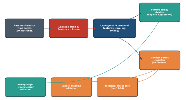
3.1 Dataset
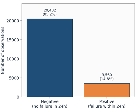
The dataset used in this study is synthetic and was constructed to resemble multi-sensor condition-monitoring data from a small industrial fleet; it does not originate from a real industrial deployment and no claim of real-world validation is made anywhere in this study. It comprises 24,042 timestamped observations from 20 machines of four types (Pump, Robotic Arm, Compressor, CNC; five machines per type), collected irregularly (median inter-observation interval approximately 16 minutes; minimum 2 minutes; maximum approximately 19 hours) over the period 2024-01-01 00:00:00 to 2024-01-14 23:59:38, a span of just under 14 days. Five continuous sensor channels are recorded per observation (vibration RMS, motor temperature, average phase current, pressure, and rotational speed), together with operating mode, hours since last maintenance, and ambient temperature. The binary target, failure within 24 hours, is positive for 3,560 observations (14.8%) and negative for the remaining 20,482 (85.2%), corresponding to 38 discrete failure episodes distributed across the 20 machines. Missing values occur only in the five raw sensor channels, at rates of 2.2% to 4.2% per channel, and were found on inspection to be unrelated to the target class, the machine identifier, or the operating mode, consistent with values missing largely at random rather than informatively. No duplicate records were present.
3.2 Data Preprocessing
Observations were sorted by machine identifier and then by timestamp to establish a strict chronological order within each machine before any temporal feature was constructed. Machine type was one-hot encoded. Categorical operating-mode values were imputed with the most frequent category and one-hot encoded within a scikit-learn pipeline; numeric sensor values were imputed with the per-feature median and standardized within the same pipeline, so that imputation and scaling parameters were always fit on training data only and applied, not refit, to validation and test partitions.
3.3 Leakage Prevention
An initial exploratory model, evaluated on a single chronological 70/15/15 train/validation/test split, achieved a receiver operating characteristic area under the curve of 1.00 and a precision-recall area under the curve of 0.9999998. This result triggered a structured leakage audit rather than being reported as a finding. The audit traced every candidate feature back to its construction and identified five variables that were excluded from all subsequent modeling because they encode information that would not be available at the moment a real-time prediction is required: rul_hours (a continuous countdown to failure); failure_type and estimated_repair_cost (both determined only once a failure event has occurred or been diagnosed); and two engineered variables, failure_start and failure_episode, used internally to construct the failure-episode structure of the dataset. In addition, five binary variables (failure_6h, failure_12h, failure_24h, failure_48h, failure_72h) were found to be direct algebraic thresholds of rul_hours (for example, failure_6h = 1 if and only if rul_hours <= 6) and were likewise excluded; these were the features responsible for the spurious perfect discrimination in the initial exploratory model, since a variable that is itself a coarsened version of the time-to-failure countdown trivially predicts a failure-within-24-hours target. Following exclusion of these variables, all subsequent feature engineering and modeling used only raw sensor and context variables observable at or before the prediction timestamp, together with temporal transformations of those variables computed using only past observations for a given machine (Section 3.4).
3.4 Temporal Feature Engineering
Two temporal representations were constructed over the course of the study. An initial representation computed lag features via per-machine shifting and rolling statistics via a fixed window of 12 observations, labeled as one-hour statistics. Because the sampling interval is irregular, a fixed-count window does not correspond to a fixed time duration, and this representation was superseded before the final ablation and modeling stage by a timestamp-aware representation, which we describe here and which is the only representation used in the reported ablation, chronological validation, unseen-machine, and stress-test results.
For each of the five sensor channels, two lag features were constructed using per-machine, timestamp-ordered shifts: lag-1 (the immediately preceding observation for that machine) and lag-6 (the observation six positions earlier for that machine). Because the sampling interval is irregular, both lags are observation-based rather than fixed-time-interval features; lag-6 does not correspond to a fixed elapsed time (for example, six hours) and is not interpreted as such anywhere in this study. Rolling statistics (mean, standard deviation, and maximum) were computed using a genuine one-hour, timestamp-indexed trailing window per machine (pandas.rolling("1h") applied to a timestamp-indexed series), verified by inspection against raw timestamps for representative rows to confirm that the window used the correct set of preceding observations within the trailing hour rather than a fixed observation count. First differences and percentage changes relative to the immediately preceding observation were also computed per machine (change features). Finally, five binary indicators flagging missingness in each raw sensor channel were constructed (missingness features). The resulting candidate feature families were: raw/context (11 features, including one-hot machine type, operating mode, hours since maintenance, and ambient temperature), lag (10 features: lag-1 and lag-6 for each of five sensors), rolling (15 features: mean, standard deviation, and maximum for each of five sensors), change (10 features: first difference and percentage change for each of five sensors), and missingness (5 features). The final feature set used for the deployed model (Section 3.6) comprises the raw/context, lag, and rolling families only (36 features); change and missingness features were evaluated in the ablation described in Section 3.5 but excluded from the final model on the basis of that ablation’s results.
3.5 Feature Ablation
To assess the incremental value of each temporal feature family, five nested feature configurations were evaluated using a logistic regression classifier (class-weighted, L2-regularized, max_iter=2000, random_state=42) across four chronological (rolling-origin) folds: (A) raw/context only, (B) raw + lag, (C) raw + lag + rolling, (D) raw + lag + rolling + change, and (E) raw + lag + rolling + change + missingness (the full 51-feature set). This ablation used logistic regression throughout, not the Random Forest model reported in Sections 3.6 to 4.5; it was intended as a lightweight, well-understood probing model for isolating the contribution of each feature family rather than as a validation of the deployed classifier.
3.6 Predictive Model
The final classifier is a Random Forest (scikit-learn RandomForestClassifier, 400 trees, unrestricted maximum depth, minimum samples per leaf of 2, balanced class weighting, random_state=42), trained on the 36-feature raw + lag + rolling representation described in Section 3.4. A decision threshold of 0.333 was selected for converting predicted probabilities into binary decisions; this threshold reflects a design choice favoring higher recall given the asymmetric cost of a missed early-warning failure relative to a false alarm, rather than the output of a formal cost-optimization or calibration procedure.
3.7 Validation Strategy
Four evaluation designs were used in this study, each targeting a different generalization question. Random train-test splitting was used only in the initial exploratory stage described in Section 3.3, where it was found to be uninformative once leakage was identified, and is not used in any reported result beyond that section. Rolling-origin (chronological, expanding-window) validation, in which each fold’s training data precedes its test data in time and successive folds extend the training window forward, was used for the feature-family ablation (Section 3.5) with the logistic regression baseline. Unseen-machine validation, in which 15 of the 20 machines (a random 75% split at the machine level, random_state=42) formed the training set and the remaining 5 machines (identifiers 1, 2, 9, 16, and 18) were withheld entirely, meaning no observation from these five machines was seen during training, was used to evaluate the final Random Forest model’s ability to generalize to assets outside its training population. Historical stress testing, in which the Random Forest model was trained on all observations before 2024-01-13 and evaluated exclusively on the final two days of the observation window (2024-01-13 to 2024-01-14), was used to assess performance under a later, non-overlapping temporal segment. We emphasize that the final Random Forest model was evaluated using a single unseen-machine split and a single stress-test split, not repeated or k-fold machine-level validation; the multi-fold chronological evidence in Section 4.3 pertains to the logistic-regression ablation only. This distinction, and its implications, is discussed further in Sections 5 and 6.
3.8 Evaluation Metrics
Discrimination was assessed using the area under the receiver operating characteristic curve (ROC-AUC), which summarizes the trade-off between true positive rate and false positive rate across all thresholds, and the area under the precision-recall curve (PR-AUC), which summarizes the trade-off between precision (the proportion of positive predictions that are correct) and recall (the proportion of true positives identified) and is generally regarded as more informative than ROC-AUC under the class imbalance present in this dataset, since it does not credit a classifier for a large true-negative count that is easy to achieve when negatives vastly outnumber positives [41][46]. At the selected decision threshold, we additionally report precision, recall, specificity (true negative rate), and F1-score (the harmonic mean of precision and recall), together with the full confusion matrix. Calibration error was assessed using the Brier score, the mean squared difference between predicted probability and the binary outcome, which is the only calibration-related quantity computed in this study; no calibration curve, reliability diagram, recalibration procedure, or conformal prediction interval was constructed (Section 6).
4. Results
4.1 Dataset Characteristics
| Characteristic | Value |
|---|---|
| Observations | 24,042 |
| Machines | 20 |
| Machine types | 4 (Pump, Robotic Arm, Compressor, CNC; 5 each) |
| Observation period | 2024-01-01 to 2024-01-14 (13d 23h 59m) |
| Median inter-observation interval | ~16 minutes (irregular; min 2 min, max ~19h 23m) |
| Sensor channels | 5 (vibration RMS, motor temperature, phase current, pressure, RPM) |
| Target | failure_within_24h (binary) |
| Positive rate | 14.8% (3,560 / 24,042) |
| Failure episodes | 38, across 20 machines |
| Missingness (sensor channels) | 2.2%-4.2% per channel; unrelated to target, machine, or operating mode |
| Duplicate records | 0 |
4.2 Feature Groups
| Family | Description | Count |
|---|---|---|
| Raw / context | Raw sensor values, operating mode, hours since maintenance, ambient temperature, one-hot machine type | 11 |
| Lag | Lag-1 and lag-6 (observation-based, not fixed time interval) per sensor | 10 |
| Rolling | Timestamp-aware 1-hour mean, standard deviation, maximum per sensor | 15 |
| Change | First difference and percentage change per sensor | 10 |
| Missingness | Binary missingness indicator per sensor | 5 |
| Final model feature set (raw + lag + rolling) | 36 | |
| Full ablation feature set (all families) | 51 |
4.3 Feature Ablation and Chronological Validation
The feature-family ablation, run with logistic regression across four chronological folds, showed that lag and rolling features accounted for essentially all of the incremental discrimination gained over the raw/context baseline, with change and missingness features contributing no further improvement within the precision of the estimate.
| Feature set | Features | ROC-AUC | PR-AUC |
|---|---|---|---|
| A. Raw / context | 11 | 0.946 ± 0.008 | 0.821 ± 0.052 |
| B. Raw + lag | 21 | 0.967 ± 0.011 | 0.892 ± 0.038 |
| C. Raw + lag + rolling | 36 | 0.978 ± 0.012 | 0.923 ± 0.040 |
| D. Raw + lag + rolling + change | 46 | 0.978 ± 0.011 | 0.923 ± 0.040 |
| E. Full + missingness | 51 | 0.978 ± 0.012 | 0.923 ± 0.040 |
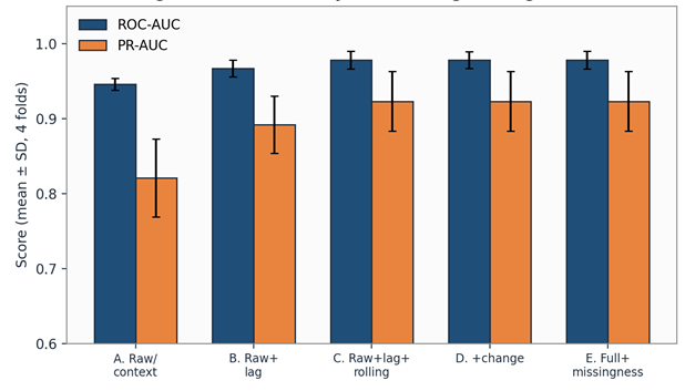
The per-fold results for the full 51-feature configuration (identical to configuration C to three decimal places, and the configuration reported here for completeness as the rolling-origin validation result) are shown in Table 4.
| Fold | ROC-AUC | PR-AUC | Precision | Recall | Specificity | F1 | Brier |
|---|---|---|---|---|---|---|---|
| 1 | 0.995 | 0.975 | 0.840 | 0.961 | 0.968 | 0.897 | 0.025 |
| 2 | 0.971 | 0.881 | 0.731 | 0.892 | 0.950 | 0.804 | 0.048 |
| 3 | 0.972 | 0.928 | 0.825 | 0.863 | 0.951 | 0.844 | 0.052 |
| 4 | 0.974 | 0.906 | 0.788 | 0.831 | 0.951 | 0.809 | 0.052 |
| Mean ± SD | 0.978 ± 0.012 | 0.923 ± 0.040 | 0.796 ± 0.043 | 0.887 ± 0.056 | 0.955 ± 0.009 | 0.838 ± 0.043 | 0.044 ± 0.013 |
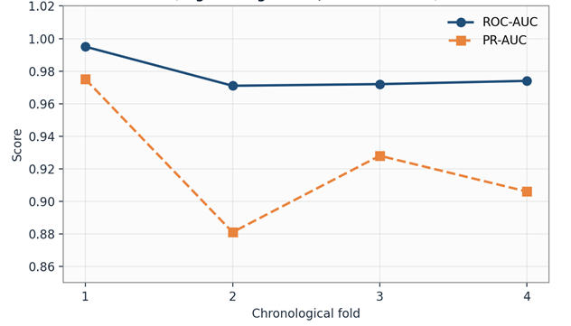
We note explicitly that Tables 3 and 4 report the performance of the logistic-regression probing model, not the Random Forest classifier described in Section 3.6. No equivalent multi-fold chronological evaluation of the Random Forest model was performed in this study.
4.4 Unseen-Machine Generalization
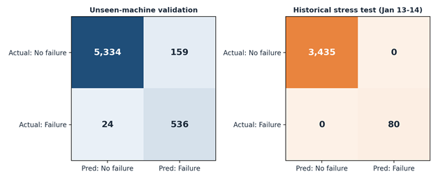
The final Random Forest model, trained on 15 machines (17,989 observations, 16.68% positive) and evaluated on 5 machines withheld entirely from training (machines 1, 2, 9, 16, 18; 6,053 observations, 9.25% positive), achieved strong discrimination and a reasonable balance of precision and recall at the 0.333 decision threshold.
| Metric | Value |
|---|---|
| ROC-AUC | 0.994 |
| PR-AUC | 0.951 |
| Brier score | 0.026 |
| Precision | 0.771 |
| Recall | 0.957 |
| Specificity | 0.971 |
| F1 | 0.854 |
| Confusion matrix (TN / FP / FN / TP) | 5,334 / 159 / 24 / 536 |
An additional analysis intended to break down unseen-machine performance by machine type did not execute successfully (the code referenced a column that had already been transformed out of the modeling dataframe at that point in the pipeline) and produced no usable output; consequently, no claim about performance differences across machine types is made in this study.
4.5 Historical Stress Testing
Training the Random Forest model on all observations before 2024-01-13 and evaluating on the final two days of the observation window (3,515 observations, 80 positive, 2.28% positive rate) produced perfect discrimination and perfect classification at the operating threshold.
| Metric | Value |
|---|---|
| ROC-AUC | 1.000 |
| PR-AUC | 1.000 |
| Brier score | 0.001 |
| Precision | 1.000 |
| Recall | 1.000 |
| Specificity | 1.000 |
| F1 | 1.000 |
| Confusion matrix (TN / FP / FN / TP) | 3,435 / 0 / 0 / 80 |
This result should not be read as evidence of near-perfect real-world reliability. It is based on 80 positive observations concentrated in a small subset of the 20 machines during a single two-day window drawn from a 14-day synthetic dataset, and a single mislabeled or unusually placed observation in a dataset this size and this imbalanced would materially change the reported metrics. We treat this result as dataset-specific evidence that the model’s discrimination did not collapse in the later period of the observation window, not as a general reliability claim.
| Parameter | Value |
|---|---|
| Algorithm | Random Forest classifier (scikit-learn) |
| Number of trees | 400 |
| Maximum depth | Unrestricted |
| Minimum samples per leaf | 2 |
| Class weighting | Balanced |
| Random state | 42 |
| Feature set | Raw + lag + rolling (36 features) |
| Decision threshold | 0.333 |
4.6 Interpretability Analysis
The only interpretability analysis performed in this study is a coefficient audit of the logistic-regression ablation model: standardized coefficients were ranked by absolute magnitude and separated into features associated with an increased versus decreased predicted probability of failure. No SHAP analysis, permutation importance analysis, or Random Forest native feature-importance extraction was performed at any point in this study. Consequently, no claim is made about which features drive the deployed Random Forest model’s predictions; the interpretability evidence available pertains only to the linear diagnostic model used in the ablation.
5. Discussion
5.1 Effect of Temporal Features
The ablation results in Table 3 indicate that the ability to represent recent trajectory, through lag and rolling statistics, rather than only the instantaneous sensor reading, accounts for essentially the entire measured improvement over the raw/context baseline. This is broadly consistent with the intuition behind condition-based maintenance: a single vibration or temperature reading close to a nominal operating range may still occur shortly before failure if the underlying trend is degrading, and a feature representation that only sees the instantaneous value cannot distinguish a stable reading from one that arrived at the end of a rising trend. That change (first-difference and percentage-change) and missingness-indicator features added no measurable further improvement in this dataset may reflect that the rolling statistics already captured the relevant short-term dynamics, that the specific synthetic degradation process used to generate this dataset does not manifest strongly in instantaneous rates of change, or simply that with only 24,042 observations and a positive rate of under 15%, the ablation lacked the statistical power to detect a small additional effect. We are not in a position to distinguish between these explanations from the present experiments and note this as an open question rather than a settled finding.
5.2 Temporal Robustness
The chronological (rolling-origin) validation in Table 4 shows relatively stable, though not identical, performance across four folds for the logistic-regression probing model, which is consistent with the broader literature’s finding that out-of-time evaluation, while typically more conservative than random splitting, need not show catastrophic degradation when the underlying data-generating process is reasonably stationary over the evaluation window [21][24]. We emphasize again that this evidence pertains to the logistic-regression model used for feature-family probing, and that no equivalent multi-fold chronological result exists for the Random Forest model that was ultimately selected as the deployed classifier; the historical stress test in Table 6 is the only chronologically later-period evidence available for that model, and it comprises a single fold rather than a distribution over folds.
5.3 Cross-Machine Generalization
The unseen-machine result in Table 5 is, in our judgment, the single most informative result in this study, because it directly targets the failure mode that random splitting cannot expose: a model that has memorized machine-specific quirks rather than learned a transferable degradation signature would be expected to degrade substantially when evaluated on machines it has never seen. That the Random Forest model retained a PR-AUC of 0.951 and a recall of 0.957 on five entirely withheld machines is a meaningful, if narrow, piece of evidence that the leakage-safe temporal features carry information that is not purely machine-specific. It demonstrates promising cross-machine generalization within this synthetic fleet of 20 machines and four machine types; it does not demonstrate that the model would generalize to a machine type outside the four represented here, to a different sensor suite, or to a real industrial deployment, and the attempted further breakdown by machine type could not be completed due to a pipeline error, so no claim is made about whether generalization was uniform across the four machine types represented in the dataset.
5.4 Interpretation and Reliability
Perfect discrimination on the historical stress test (Section 4.5) illustrates a general hazard in reporting predictive maintenance results under class imbalance: with only 80 positive observations concentrated in a subset of machines, a result of this kind is highly sensitive to the specific composition of the evaluation window and should not be extrapolated into a claim of near-perfect real-world reliability. This aligns with a broader caution in the imbalanced-classification literature that a single scalar summary metric, however favorable, can obscure how few positive examples that summary is actually built from [41][46]. On interpretability, the coefficient audit available in this study offers, at best, a partial and model-specific account of what the logistic-regression baseline is responding to; it does not license any claim about the reasoning of the deployed Random Forest model, and we regard the addition of a genuine SHAP or permutation-importance analysis of that model as one of the more valuable and inexpensive extensions of this work. On calibration and uncertainty, the Brier scores reported in Tables 4, 5, and 6 provide some indication of probabilistic accuracy, but the conformal-prediction and calibrated-threshold procedure that was specified during the design of this study (a target threshold of 0.333 alongside a stated 90% target coverage) was not implemented; no coverage was measured, and no prediction interval was constructed. We treat this as a design intention that remains future work rather than as a completed contribution.
5.5 Implications for Predictive Maintenance
These results support a narrower and more defensible conclusion than the framing with which many predictive maintenance studies open. The evidence here supports the claim that leakage-aware temporal feature engineering improves early failure detection, evaluated chronologically, for a linear probing model, and that a Random Forest classifier built on the same leakage-safe features retains strong discrimination on both a single later time period and a single set of machines withheld from training. It does not support a claim of validated real-time deployment, of remaining-useful-life estimation, of a completed explainability pipeline for the deployed model, or of calibrated uncertainty quantification. For practitioners, the practical implication is that the methodological ingredients used here, leakage auditing, chronological validation, and machine-level holdout, are inexpensive to apply relative to the risk of reporting an inflated benchmark result, and that a genuinely deployment-ready predictive maintenance system would need to close each of the specific gaps identified in Section 6 before the stronger claims implied by the original framing of this research question could be responsibly made.
6. Limitations
This study has several limitations that bear directly on how its results should be interpreted.
Validation scope. An important limitation concerns the number of independent holdout evaluations performed with the final Random Forest model. Although temporal feature configurations were examined through rolling-origin validation, the final Random Forest model was evaluated using a single unseen-machine holdout and a single later-period temporal stress-test split, rather than repeated or k-fold machine-level validation. Consequently, the observed cross-machine and temporal generalization results should be interpreted as evidence under the specific evaluation splits used in this study, rather than as estimates of performance variability across a broad population of machines or operating environments. The unseen-machine evaluation is particularly informative because the test machines were not represented in the training set, but the experiment still involves only a limited number of held-out machines. Similarly, the perfect performance observed during the January 13-14 stress test should not be interpreted as evidence of universally perfect predictive performance. The positive cases in this period were concentrated in a small subset of machines, and the underlying dataset covers only a short synthetic observation period. Additional repeated machine-level validation, longer temporal evaluation windows, and external validation using real industrial telemetry would be necessary to establish the stability and transferability of the findings more broadly.
Synthetic data. The dataset is synthetic and was not collected from an operating industrial facility. While synthetic construction allows the leakage and validation-design questions central to this study to be examined without the confound of unverified real-world ground truth, and while synthetic data generation is an established and actively developed strategy in the predictive maintenance literature for addressing the scarcity of labeled failure data [47][51], it also means that no aspect of this study constitutes evidence of performance on real sensor data, and the specific numerical results reported here should not be assumed to transfer to any other dataset, synthetic or real.
Short observation window and small machine population. The dataset spans only 14 days and 20 machines across four types, with 38 total failure episodes. This is a small basis from which to draw conclusions about generalization across machine types, seasonal or long-term operating variation, or rare failure modes not represented in the observed episodes.
Temporal correlation and single-seed evaluation. All modeling used a single random seed (random_state=42) throughout. No repeated-seed variance estimation was performed for the Random Forest model; the only variance estimate available in this study (the standard deviation across four chronological folds) pertains to the logistic-regression ablation.
No remaining-useful-life modeling. The rul_hours variable was examined only for its leakage relationship to the target and was never used as a regression target. This study establishes evidence for early binary failure detection only, not for remaining-useful-life estimation, and the two should not be conflated.
Incomplete interpretability. Only a coefficient audit of a logistic-regression baseline was performed. No SHAP, permutation-importance, or native feature-importance analysis of the deployed Random Forest model was conducted.
Incomplete calibration and uncertainty quantification. A conformal-prediction and coverage-evaluation procedure was specified during the design of this study but was not implemented; Brier scores are the only calibration-related evidence available, and no calibrated probability, coverage guarantee, or prediction interval was produced or evaluated.
No external or real-world validation. No aspect of this study was evaluated against real industrial telemetry, and no claim of real-world deployment validity is made.
7. Conclusion
This study asked how a leakage-aware temporal feature representation affects early industrial failure detection under chronological and machine-level evaluation, using a synthetic 20-machine sensor dataset. An initial exploratory model achieved spuriously perfect discrimination through features that were, on inspection, direct algebraic derivatives of a time-to-failure countdown variable; removing these and constructing a leakage-safe representation of raw sensor values, observation-based lags, and timestamp-aware rolling statistics yielded a feature-family ablation in which lag and rolling information accounted for essentially all of the measured gain over instantaneous readings alone. A Random Forest classifier built on this leakage-safe representation retained strong discrimination, ROC-AUC of 0.994 and PR-AUC of 0.951, on five machines withheld entirely from training, and reproduced strong, though dataset-specific and not generalizable, discrimination during a later two-day stress-testing window. The methodological contribution of this work is not a new classifier but a transparent accounting of what a leakage-aware, dual-validation predictive maintenance pipeline can and cannot demonstrate: it distinguishes benchmark evidence, present here in the form of chronological and unseen-machine evaluation, from deployment evidence, which would additionally require multi-fold validation of the deployed model, completed calibration and uncertainty quantification, model-specific interpretability analysis, and evaluation on real industrial telemetry, none of which were completed in this study. The next scientific step is not a more elaborate model but closure of these specific evidentiary gaps against the same or a comparable dataset, followed, only once that closure is achieved, by evaluation against real sensor data from an operating industrial system.
Declarations
Ethics Approval
Not applicable. This study did not involve human participants or animals; all data are synthetic sensor readings generated to resemble industrial condition-monitoring data.
Informed Consent
Not applicable. No human participants were involved in this study.
Conflict of Interest
The authors declare no conflict of interest.
Funding
This research received no specific grant or funding from any funding agency in the public, commercial, or not-for-profit sectors.
Data Availability
The synthetic dataset and analysis code generated for this study are available at https://github.com/TMF1212/Leakage-Aware-Temporal-Feature-Engineering-for-Early-Industrial-Failure-Detection.
Use of AI Tools
Grammarly was used to check the manuscript for grammatical errors, and Quillbot was used to check the manuscript for plagiarism. No generative AI tool was used to author, generate, or substantively rewrite the manuscript text, analysis, or code.
Author Contributions
M.O.F. formulated the problem statement, proofread the manuscript, and supervised the study. D.O.O. conducted the data analysis. T.I.A. and V.O.O. contributed to conceptualization. G.O.O. developed the methodology. All authors reviewed and approved the final manuscript.
References
- Benmansour, O., Medarhri, I., & Hosni, M. (2026). Predictive maintenance in Industrial Systems Using Machine Learning: A Review. Statistics, Optimization & Information Computing, 15(4). DOI ↗ Google Scholar ↗
- Tsallis, C., et al. (2025). Application-Wise Review of Machine Learning-Based Predictive Maintenance: Trends, Challenges, and Future Directions. Applied Sciences. DOI ↗ Google Scholar ↗
- Leukel, J., González, J., & Riekert, M. (2021). Adoption of machine learning technology for failure prediction in industrial maintenance: A systematic review. Journal of Manufacturing Systems, 61, 87-96. DOI ↗ Google Scholar ↗
- Li, W., et al. (2025). Comparison of deep learning models for predictive maintenance in industrial manufacturing systems using sensor data. Scientific Reports. Google Scholar ↗
- Guidotti, D., et al. (2025). A Systematic Literature Review of Supervised Machine Learning Techniques for Predictive Maintenance in Industry 4.0. IEEE Access. Google Scholar ↗
- Benhanifia, A., et al. (2025). Systematic review of predictive maintenance practices in the manufacturing sector. Intelligent Systems with Applications. DOI ↗ Google Scholar ↗
- Wu, X., et al. (2024). Review of Machine Learning Algorithms for Predictive Maintenance in Industrial Applications. 2024 8th International Conference on Electrical, Mechanical and Computer Engineering (ICEMCE). Google Scholar ↗
- Azari, M. S., Flammini, F., Santini, S., & Caporuscio, M. (2023). A Systematic Literature Review on Transfer Learning for Predictive Maintenance in Industry 4.0. IEEE Access, 11, 12887-12910. Google Scholar ↗
- Hector, I., & Panjanathan, R. (2024). Predictive maintenance in Industry 4.0: a survey of planning models and machine learning techniques. PeerJ Computer Science, 10, e2016. DOI ↗ Google Scholar ↗
- Elkateb, S. N., et al. (2024). Machine learning and IoT-based predictive maintenance approach for industrial applications. Alexandria Engineering Journal. Google Scholar ↗
- Albelali, S., et al. (2025). Hidden Leaks in Time Series Forecasting: How Data Leakage Affects LSTM Evaluation Across Configurations and Validation Strategies. arXiv preprint. Google Scholar ↗
- Kapoor, S., & Narayanan, A. (2023). Leakage and the reproducibility crisis in machine-learning-based science. Patterns, 4(9), 100804. Google Scholar ↗
- Apicella, A., Isgrò, F., Prevete, R., et al. (2024). Don’t push the button! Exploring data leakage risks in machine learning and transfer learning. Artificial Intelligence Review. DOI ↗ Google Scholar ↗
- Bernett, J., Blumenthal, D. B., Grimm, D. G., Haselbeck, F., Joeres, R., Kalinina, O. V., et al. (2024). Guiding questions to avoid data leakage in biological machine learning applications. Nature Methods, 21, 1444-1453. DOI ↗ Google Scholar ↗
- Sasse, L., Nicolaisen-Sobesky, E., Dukart, J., Eickhoff, S. B., Götz, M., Hamdan, S., et al. (2025). Overview of leakage scenarios in supervised machine learning. Journal of Big Data, 12, Article 135. DOI ↗ Google Scholar ↗
- Yang, X., Li, J., & Jiang, X. (2024). Research on information leakage in time series prediction based on empirical mode decomposition. Scientific Reports, 14, Article 28362. DOI ↗ Google Scholar ↗
- Liu, F., Chen, Y., & Zhao, J. (2022). A Prediction Method with Data Leakage Suppression for Time Series. Electronics, 11(22), Article 3701. DOI ↗ Google Scholar ↗
- Cerqua, A., Di Stefano, R., Letta, M., & Miranda, S. (2025). On the (Mis)Use of Machine Learning With Panel Data. Oxford Bulletin of Economics and Statistics, 88(3), 506-518. DOI ↗ Google Scholar ↗
- Schnur, C., Goodarzi, P., Robin, Y., Schauer, J., & Schütze, A. (2025). A Machine Learning Dataset of Artificial Inner Ring Damage on Cylindrical Roller Bearings Measured Under Varying Cross-Influences. Data, 10(5), Article 77. DOI ↗ Google Scholar ↗
- Goodarzi, P., Schütze, A., & Schneider, T. (2025). Domain shifts in industrial condition monitoring: a comparative analysis of automated machine learning models. Journal of Sensors and Sensor Systems, 14(2), 119-132. DOI ↗ Google Scholar ↗
- Maldonado, S., López, J., & Iturriaga, A. (2022). Out-of-time cross-validation strategies for classification in the presence of dataset shift. Applied Intelligence, 52, 5770-5783. DOI ↗ Google Scholar ↗
- Hewamalage, H., Ackermann, K., & Bergmeir, C. (2023). Forecast evaluation for data scientists: common pitfalls and best practices. Data Mining and Knowledge Discovery, 37, 788-832. DOI ↗ Google Scholar ↗
- Allgaier, J., & Pryss, R. (2024). Cross-Validation Visualized: A Narrative Guide to Advanced Methods. Machine Learning and Knowledge Extraction, 6(2), 1378-1388. DOI ↗ Google Scholar ↗
- Hespeler, S. C., Moriano, P., Li, M., & Hollifield, S. C. (2025). Temporal cross-validation impacts multivariate time series subsequence anomaly detection evaluation. arXiv preprint arXiv:2506.12183. DOI ↗ Google Scholar ↗
- Jang, K., Pilario, K. E. S., Lee, N., Moon, I., & Na, J. (2025). Explainable Artificial Intelligence for Fault Diagnosis of Industrial Processes. IEEE Transactions on Industrial Informatics, 21(1), 4-11. DOI ↗ Google Scholar ↗
- Gawde, S., Patil, S., Kumar, S., Kamat, P., Kotecha, K., & Alfarhood, S. (2024). Explainable Predictive Maintenance of Rotating Machines Using LIME, SHAP, PDP, ICE. IEEE Access, 12, 29345-29361. DOI ↗ Google Scholar ↗
- Wang, L., & Wu, M. (2025). Research on bearing fault diagnosis based on machine learning and SHAP interpretability analysis. Scientific Reports, 15, Article 41242. DOI ↗ Google Scholar ↗
- Brusa, E., Cibrario, L., Delprete, C., & Di Maggio, L. G. (2023). Explainable AI for Machine Fault Diagnosis: Understanding Features’ Contribution in Machine Learning Models for Industrial Condition Monitoring. Applied Sciences, 13(4), Article 2038. DOI ↗ Google Scholar ↗
- Sharma, J., Mittal, M. L., & Soni, G. (2025). Predictive Maintenance of Industrial Assets: A Fault Detection and Diagnosis Approach with Explainable AI. International Journal of Reliability, Quality and Safety Engineering, 32(2), Article 2440007. DOI ↗ Google Scholar ↗
- Cohen, J., Huan, X., & Ni, J. (2024). Shapley-based explainable AI for clustering applications in fault diagnosis and prognosis. Journal of Intelligent Manufacturing, 35, 4071-4086. DOI ↗ Google Scholar ↗
- Ahangar, M. N., Farhat, Z. A., Sivanathan, A., Ketheesram, N., & Kaur, S. (2026). Explainable AI-Driven Quality and Condition Monitoring in Smart Manufacturing. Sensors, 26(3), Article 911. DOI ↗ Google Scholar ↗
- Filho, T. S., Song, H., Perello-Nieto, M., Santos-Rodriguez, R., Kull, M., & Flach, P. (2023). Classifier calibration: a survey on how to assess and improve predicted class probabilities. Machine Learning, 112, 3211-3260. DOI ↗ Google Scholar ↗
- Angelopoulos, A. N., & Bates, S. (2023). A Gentle Introduction to Conformal Prediction and Distribution-Free Uncertainty Quantification. arXiv preprint arXiv:2107.07511. DOI ↗ Google Scholar ↗
- Einbinder, B.-S., Romano, Y., Sesia, M., & Zhou, Y. (2022). Training Uncertainty-Aware Classifiers with Conformalized Deep Learning. Advances in Neural Information Processing Systems 35 (NeurIPS 2022). DOI ↗ Google Scholar ↗
- Lee, D., Huang, X., Hassani, H., & Dobriban, E. (2023). T-Cal: An optimal test for the calibration of predictive models. Journal of Machine Learning Research, 24(335), 1-72. Google Scholar ↗
- van der Laan, L., & Alaa, A. M. (2024). Self-Calibrating Conformal Prediction. Advances in Neural Information Processing Systems 37 (NeurIPS 2024). DOI ↗ Google Scholar ↗
- Luo, R., & Zhou, Z. (2024). Trustworthy Classification through Rank-Based Conformal Prediction Sets. arXiv preprint arXiv:2407.04407. DOI ↗ Google Scholar ↗
- Ghosh, S., Belkhouja, T., Yan, Y., & Doppa, J. R. (2023). Improving Uncertainty Quantification of Deep Classifiers via Neighborhood Conformal Prediction. Proceedings of the AAAI Conference on Artificial Intelligence, 37(6), 7722-7730. DOI ↗ Google Scholar ↗
- Ahangar, M. N., et al. (2025). AI Trustworthiness in Manufacturing: Challenges, Toolkits, and the Path to Industry 5.0. Sensors, 25. DOI ↗ Google Scholar ↗
- Lv, Z., Chen, D., Lou, R., & Wang, Q. (2021). Trustworthiness in Industrial IoT Systems Based on Artificial Intelligence. IEEE Transactions on Industrial Informatics, 17(2), 1496-1504. DOI ↗ Google Scholar ↗
- Martin, B., Bennett, T. D., DeWitt, P. E., Russell, S., & Sanchez-Pinto, L. N. (2025). Use of the Area Under the Precision Recall Curve to Evaluate Prediction Models of Rare Critical Illness Events. Pediatric Critical Care Medicine, 26(6), e855-e859. DOI ↗ Google Scholar ↗
- Richardson, E., Trevizani, R., Greenbaum, J. A., Carter, H., Nielsen, M., & Peters, B. (2024). The receiver operating characteristic curve accurately assesses imbalanced datasets. Patterns, 5(6), 100994. DOI ↗ Google Scholar ↗
- Imani, M., Joudaki, M., Bagheri, A., & Arabnia, H. R. (2026). Why ROC-AUC Is Misleading for Highly Imbalanced Data: In-Depth Evaluation of MCC, F2-Score, H-Measure, and AUC-Based Metrics Across Diverse Classifiers. Technologies, 14(1), Article 54. DOI ↗ Google Scholar ↗
- Movahedi, F., & Antaki, J. F. (2021). Limitation of ROC in Evaluation of Classifiers for Imbalanced Data. Journal of Heart and Lung Transplantation, 40(4 Suppl), S473. DOI ↗ Google Scholar ↗
- Kim, M., & Hwang, K.-B. (2022). An empirical evaluation of sampling methods for the classification of imbalanced data. PLoS ONE, 17(7), e0271260. DOI ↗ Google Scholar ↗
- Sujon, K. M., Hassan, R., Choi, K., & Samad, M. A. (2025). Accuracy, precision, recall, f1-score, or MCC? Empirical evidence from advanced statistics, ML, and XAI for evaluating business predictive models. Journal of Big Data, 12, Article 268. DOI ↗ Google Scholar ↗
- Nieminen, W., Gebreweld, H., Liuha, A., Nissinen, M., Verdugo, M., Mikkola, A., et al. (2026). Synthetic Data for Predictive Maintenance: A Systematic Review and Framework for Industry 4.0 Applications. Journal of Intelligent Manufacturing. DOI ↗ Google Scholar ↗
- Jakubowski, J., Bobek, S., & Nalepa, G. J. (2026). Benchmark datasets for predictive maintenance challenges in steel manufacturing. Frontiers in Artificial Intelligence, 9. DOI ↗ Google Scholar ↗
- Stanton, I., Munir, K., Ikram, A., & El-Bakry, M. (2024). Data augmentation for predictive maintenance: Synthesising aircraft landing gear datasets. Engineering Reports, 6(12), e12946. DOI ↗ Google Scholar ↗
- Schwarz, A., Rodriguez Rahal, J., Sahelices, B., Barroso-García, V., Weis, R., & Duque Antón, S. (2025). Data augmentation in predictive maintenance applicable to hydrogen combustion engines: a review. Artificial Intelligence Review, 58, Article 32. DOI ↗ Google Scholar ↗
- Dzaferagic, M., Marchetti, N., & Macaluso, I. (2021). Fault Detection and Classification in Industrial IoT in Case of Missing Sensor Data. IEEE Internet of Things Journal, 9(11), 8892-8900. DOI ↗ Google Scholar ↗
- Ferreira, C., & Gonçalves, G. (2022). Remaining Useful Life prediction and challenges: A literature review on the use of Machine Learning Methods. Journal of Manufacturing Systems, 63, 550-562. DOI ↗ Google Scholar ↗
- Wu, F., Wu, Q., Tan, Y., & Xu, X. (2024). Remaining Useful Life Prediction Based on Deep Learning: A Survey. Sensors, 24(11), Article 3454. DOI ↗ Google Scholar ↗
- Ovacıklı, A. K., Yagcioglu, M., Demircioglu, S., Kocatekin, T., & Birtane, S. (2025). Supervised Learning-Based Fault Classification in Industrial Rotating Equipment Using Multi-Sensor Data. Applied Sciences, 15(13), Article 7580. DOI ↗ Google Scholar ↗
- Alghtus, K. M. A., Gannan, A., Alhajri, K. M., Al Jubouri, A. L. A., & Al-Janahi, H. A. I. (2025). AI-Powered Machine Learning Approaches for Fault Diagnosis in Industrial Pumps. arXiv preprint arXiv:2508.15550. DOI ↗ Google Scholar ↗
- Koldasbayeva, D., & Zaytsev, A. (2025). Foundation for unbiased cross-validation of spatio-temporal models for species distribution modeling. Ecological Informatics. DOI ↗ Google Scholar ↗
- Kingphai, K., Kanjina, P., Sanittham, K., & Wongsanurak, W. (2026). Adaptive Cross-Validation Under Concept Drift for Time Series Forecasting. Journal of Computer Science, 22(7), 2104-2117. DOI ↗ Google Scholar ↗